
2024-06-13
The notebook for this post can be found here.
In the previous post of this series, we introduced the problem of Malaria detection and prepared and preprocessed our dataset. Now, let’s build and train a few deep-learning models to see if we can detect Malaria with good accuracy and recall.
We’ll start with a CNN model as our baseline:
def build_base_model():
 set_seed()
 model = Sequential([
 Conv2D(16, (2, 2), padding="same", activation="relu", input_shape=(64, 64, 3)),
 MaxPooling2D(pool_size=(2, 2)),
 Dropout(0.2),
 Conv2D(32, (2, 2), padding="same", activation="relu"),
 MaxPooling2D(pool_size=(2, 2)),
 Dropout(0.2),
 Conv2D(64, (2, 2), padding="same", activation="relu"),
 MaxPooling2D(pool_size=(2, 2)),
 Dropout(0.2),
 Flatten(),
 Dense(512, activation='relu'),
 Dropout(0.5),
 Dense(2, activation='softmax')
 ])
  return model

base_model = build_base_model()
base_model.compile(
  optimizer=tf.keras.optimizers.Adamax(learning_rate=0.005),
  loss='categorical_crossentropy',
  metrics=['accuracy']
)
This model uses 3 convolution layers with ReLU activation, each followed by a MaxPooling layer to reduce resolution and then a Dropout layer for regularization. We’ll train this baseline model (and all models after this)and evaluate its performance with the following code:
history_base = base_model.fit(
X_train_blur_normalized,
y_train_one_hot,
epochs=10,
validation_split=0.1,
shuffle=True,
callbacks=[checkpoint_base]
)
y_pred_base = base_model.predict(X_test_blur_normalized)
y_pred_base_classes = np.argmax(y_pred_base, axis=1)
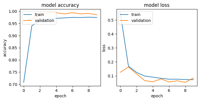
print(classification_report(y_test_np, y_pred_base_classes))Table 1. and Figure 1. show the classification report and the confusion matrix of the base_model. The training and validation curve is shown in Figure 2. While already performing quite well, our base model might benefit from adding subtler features to our cell images. Malaria parasites can manifest in various ways within a cell, and I wanted my model to capture as many of these variations as possible. This led me to experiment with deeper architectures next.
Table 1. The Classification Report of the Base Model
| Precision | Recall | F1-Score | Support | |
|---|---|---|---|---|
| Uninfected | 0.99 | 0.98 | 0.98 | 1300 |
| Parasitized | 0.98 | 0.99 | 0.98 | 1300 |
| accuracy | 0.98 | 2600 | ||
| macro Avg | 0.98 | 0.98 | 0.98 | 2600 |
| Weighted Avg | 0.98 | 0.98 | 0.98 | 2600 |
My first improvement was to add more layers to the network. The motivation here is that more layers mean more parameters and the capacity to learn complex features. I added 2 extra convolutional layers and another dense layer. The hope is that the additional convolutional layer would allow the model to detect more intricate patterns while the extra dense layer would give it more flexibility in combining these patterns for classification:
def build_model_1():
 set_seed()
 model = Sequential()
 model.add(Conv2D(16, (2, 2), padding = "same", activation = "relu", input_shape=(IMG_SIZE, IMG_SIZE, 3)))
 model.add(MaxPooling2D(pool_size=(2, 2)))
 model.add(Dropout(0.2))
 model.add(Conv2D(32, (2, 2), padding = "same", activation = "relu"))
 model.add(MaxPooling2D(pool_size=(2, 2)))
 model.add(Dropout(0.2))
 model.add(Conv2D(64, (2, 2), padding = "same", activation = "relu"))
 model.add(MaxPooling2D(pool_size=(2, 2)))
 model.add(Dropout(0.2))
 model.add(Conv2D(128, (2, 2), padding = "same", activation = "relu"))
 model.add(MaxPooling2D(pool_size=(2, 2)))
 model.add(Dropout(0.2))
 model.add(Conv2D(256, (2, 2), padding = "same", activation = "relu"))
 model.add(MaxPooling2D(pool_size=(2, 2)))
 model.add(Dropout(0.2))
 model.add(Flatten())
 model.add(Dense(512, activation='relu'))
 model.add(Dropout(0.5))
 model.add(Dense(256, activation='relu'))
 model.add(Dense(2, activation='softmax'))
Table 2. The Classification Report of Model 1
| precision | recall | f1-score | support | |
|---|---|---|---|---|
| Uninfected | 0.98 | 0.98 | 0.98 | 1300 |
| Parasitized | 0.98 | 0.98 | 0.98 | 1300 |
| accuracy | 0.98 | 2600 | ||
| macro avg | 0.98 | 0.98 | 0.98 | 2600 |
| weighted avg | 0.98 | 0.98 | 0.98 | 2600 |

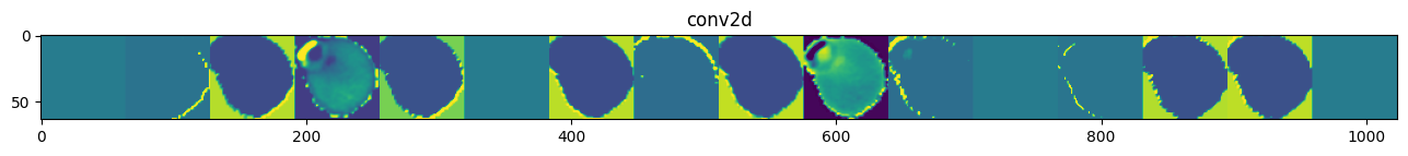
Despite being a deeper model, model_1’s performance is similar to the base_model’s. For model_1, one misclassified image has a purple shape at the boundary, which the model cannot capture well. Figure 4 shows the outputs of the first CNN layer, where many learned features are flat images. This may be caused by the ReLU activation function. We can use a different activation function to see if that improves the feature extraction and model performance. Furthermore, we can improve the training speed by stabilizing the variance of the inputs to each layer. In the next model, we employ the LeakyRelu activation and BatchNormalization:
def build_model_2():
 set_seed()
 model = Sequential()
 model.add(Conv2D(32, (2, 2), padding = "same", input_shape=(IMG_SIZE, IMG_SIZE, 3)))
 model.add(BatchNormalization())
 model.add(LeakyReLU(alpha=0.1))
 model.add(Conv2D(32, (2, 2), padding = "same"))
 model.add(BatchNormalization())
 model.add(LeakyReLU(alpha=0.1))
 model.add(MaxPooling2D(pool_size=(2, 2)))
 model.add(Dropout(0.2))
 model.add(Conv2D(64, (2, 2), padding = "same"))
 model.add(BatchNormalization())
 model.add(LeakyReLU(alpha=0.1))
 model.add(Conv2D(64, (2, 2), padding = "same"))
 model.add(BatchNormalization())
 model.add(LeakyReLU(alpha=0.1))
 model.add(MaxPooling2D(pool_size=(2, 2)))
 model.add(Dropout(0.2))
 model.add(Conv2D(128, (2, 2), padding = "same"))
 model.add(BatchNormalization())
 model.add(LeakyReLU(alpha=0.1))
 model.add(MaxPooling2D(pool_size=(2, 2)))
 model.add(Dropout(0.2))
 model.add(Conv2D(256, (2, 2), padding = "same"))
 model.add(BatchNormalization())
 model.add(LeakyReLU(alpha=0.1))
 model.add(MaxPooling2D(pool_size=(2, 2)))
 model.add(Dropout(0.2))
 model.add(Flatten())
 model.add(Dense(512))
 model.add(BatchNormalization())
 model.add(LeakyReLU(alpha=0.1))
 model.add(Dropout(0.5))
 model.add(Dense(256))
 model.add(BatchNormalization())
 model.add(LeakyReLU(alpha=0.1))
 model.add(Dense(2, activation='softmax'))

return model
Batch Normalization was motivated by the desire to reduce internal covariate shift - a fancy way of saying that the distribution of each layer’s inputs changes during training, which can slow down the learning process. By normalizing these inputs, we can train deeper networks more efficiently.
LeakyReLU, on the other hand, was an attempt to solve the “dying ReLU” problem. In standard ReLU, neurons can sometimes get stuck at 0, effectively “dying” and no longer contributing to the network. LeakyReLU allows a small gradient when the unit is not active, potentially keeping all neurons in the game.
Table 3. The Classification Report of Model 2
| Precision | Recall | F1-Score | Support | |
|---|---|---|---|---|
| Uninfected | 0.99 | 0.98 | 0.98 | 1300 |
| Parasitized | 0.98 | 0.99 | 0.98 | 1300 |
| accuracy | 0.98 | 2600 | ||
| macro avg | 0.98 | 0.98 | 0.98 | 2600 |
| weighted avg | 0.98 | 0.98 | 0.98 | 2600 |
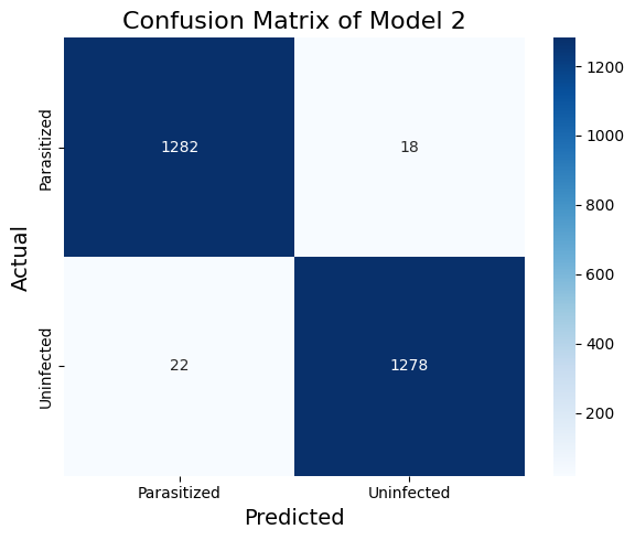
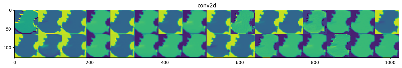
We have improved some precision and recall metrics, as shown in the classification report and the confusion matrix. The features of the first layer (Figure 6) are no longer flat like in model_1.
Despite these improvements, our model might be limited by the training data available. In medical imaging, gathering large datasets can be challenging due to privacy concerns and the cost of expert annotation. This led me to explore data augmentation techniques.
Data augmentation involves creating new training examples by applying transformations to our existing images. The motivation here is to expose our model to a wider variety of cell appearances, making it more robust to variations it might encounter in real-world scenarios.
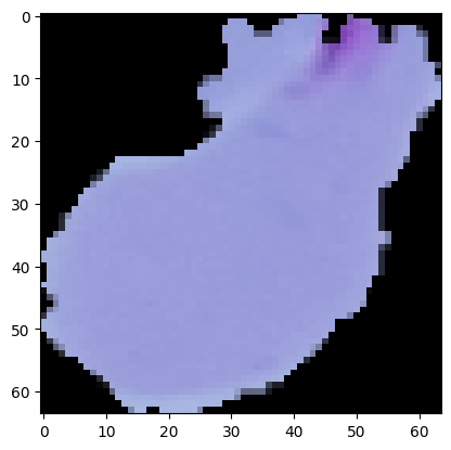
All previous models have difficulty correctly labelling an image like the one in Figure 7, where the purple stain is at the boundary of the image. However, this type of image is supposedly in the minority, making it challenging for our model to identify them. I want the model to pay more attention to this type of image.
To achieve this, I take the misclassified images in the training set and generate 4000 augmented data from these misclassified images using techniques like rotation, flipping, and zooming.
datagen = ImageDataGenerator(
rotation_range=45,
width_shift_range=0.1,
height_shift_range=0.1,
zoom_range=0.2,
horizontal_flip=True,
vertical_flip=True,
fill_mode='constant'
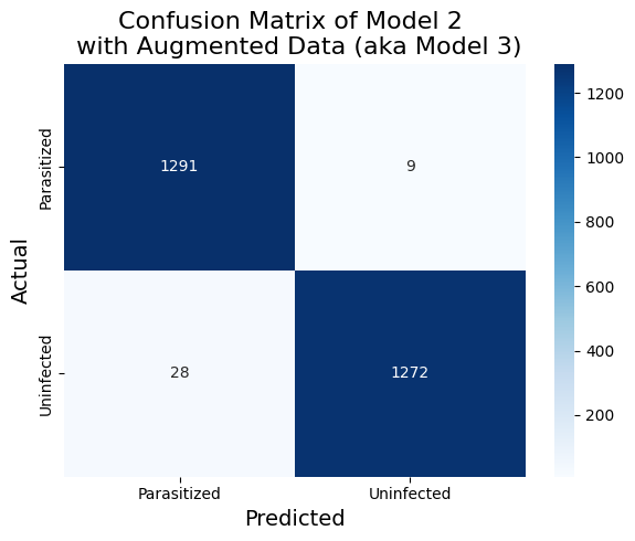
)I then take the trained model_2 above and retrain on the combined dataset of the original training data and the augmented data. The test set performance is again improved, as shown in Table 4 and Figure 8
Table 4. The Classification Report of Model 2 on Augmented Data (aka Model 3)
| precision | recall | f1-score | support | |
|---|---|---|---|---|
| Uninfected | 0.99 | 0.98 | 0.99 | 1300 |
| Parasitized | 0.98 | 0.99 | 0.99 | 1300 |
| accuracy | 0.99 | 2600 | ||
| macro avg | 0.99 | 0.99 | 0.99 | 2600 |
| weighted avg | 0.99 | 0.99 | 0.99 | 2600 |
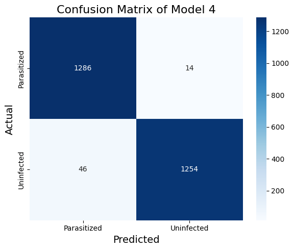
For my final experiment, I wanted to see if we could benefit from transfer learning. I wanted to leverage the power of models that have been trained on massive datasets like ImageNet. Even though these models were not trained on cell images, the low-level features they learn (like edge detection) could be valuable for our task.
I chose to use VGG16 as our base model:
from keras.applications.vgg16 import VGG16, preprocess_input
def build_model_4():
 set_seed()
 vgg16_model.trainable = False

 transfer_layer = vgg16_model.get_layer('block3_pool')
 x = Conv2D(512, (2, 2), padding = "same")(transfer_layer.output)
 x = MaxPooling2D(pool_size=(2, 2))(x)
 x = LeakyReLU(alpha=0.1)(x)
 x = Conv2D(512, (2, 2), padding = "same")(x)
 x = MaxPooling2D(pool_size=(2, 2))(x)
 x = BatchNormalization()(x)
 x = LeakyReLU(alpha=0.1)(x)
 x = Flatten()(x)
 x = Dense(512)(x)
 x = BatchNormalization()(x)
 x = LeakyReLU(alpha=0.1)(x)
 x = Dropout(0.5)(x)
 x = Dense(256)(x)
 x = BatchNormalization()(x)
 x = LeakyReLU(alpha=0.1)(x)
 x = Dropout(0.5)(x)
 pred = Dense(2, activation='softmax')(x)
 model = Model(vgg16_model.input, pred)
  return model
The idea was to use VGG16’s pre-trained weights for feature extraction and then train our own top layers for the specific task of malaria detection. This approach often leads to good performance with less training time and data.
The input to the VGG16 model differs from the ones we used for the other data. Since the input needs to be preprocessed by keras.applications.vgg16.preprocess_input, which takes RGB inputs, we pass in the original dataset from Kaggle instead of our own preprocessed data. We do this for both the training and test data.
Table 5 and Figure 9 show that a finetuned VGG16 model can achieve competitive results.
Table 5. The Classification Report of Model 4
| Precision | Recall | F1-Score | Support | |
|---|---|---|---|---|
| Uninfected | 0.99 | 0.96 | 0.98 | 1300 |
| Parasitized | 0.97 | 0.99 | 0.98 | 1300 |
| accuracy | 0.98 | 2600 | ||
| macro avg | 0.98 | 0.98 | 0.98 | 2600 |
| weighted avg | 0.98 | 0.98 | 0.98 | 2600 |
In the next post of this series, we’ll discuss the results, draw insights, and explore potential improvements to our malaria detection system. Stay tuned!