In Part 1 we derived the expected performance of a continuously rebalanced mean-reversion strategy under the assumption that the trader knows the asset’s true fair value exactly and can rebalance continuously frictionlessly. The asymptotic Sharpe ratio turned out to depend only on the speed of mean reversion \theta:

\mathrm{SR}_\infty = \sqrt{\frac{\theta}{2}}.

In practice, fair value is never observed directly and must be estimated. As a first order approximation, how does a persistent error in the fair-value estimate affect the strategy’s risk-adjusted performance?

This post answers that question first in the simplest possible setting: that the fair-value error is a known constant M. Even in this stylised case, the results are instructive:

• The expected PnL is unchanged — the bias washes out because the true mispricing is symmetric about zero.
• The risk increases — the trader holds a systematic offset position that adds path volatility.
• The Sharpe ratio degrades by a closed-form penalty factor that depends on M, \sigma, and \theta.

1 Model

We continue with our setup from Part 1. The log price is p_t = \log P_t, the true log fair value is v_t (assumed constant), and the true mispricing follows an Ornstein–Uhlenbeck process:

dX_t = -\theta X_t\, dt + \sigma\, dW_t, \qquad X_0 = 0,

so that X_t = p_t - v_t \sim \mathcal{N}(0, s_t^2) with s_t^2 = \frac{\sigma^2}{2\theta}(1 - e^{-2\theta t}).

Suppose the trader does not observe v_t directly but instead uses an estimate \tilde{v}_t that carries a constant bias M in log terms:

\tilde{v}_t = v_t + M.

The trader’s perceived mispricing is therefore

\tilde{X}_t = p_t - \tilde{v}_t = (p_t - v_t) - M = X_t - M.

When M > 0 the trader systematically under-estimates the asset’s price level (thinks it is cheaper than it really is); when M < 0 the trader over-estimates it.

The strategy trades against the estimated mispricing \tilde{X}_t. Since the fair value is constant, dp_t = dX_t, and the instantaneous PnL is

dY_t = -\tilde{X}_t\, dp_t = -(X_t - M)\, dX_t.

2 Closed-Form Terminal PnL

Splitting the PnL into the unbiased part (already computed in Part 1) and the bias-induced part:

dY_t = \underbrace{-X_t\, dX_t}_{\text{Part 1}} + \underbrace{M\, dX_t}_{\text{bias term}}.

Integrating from 0 to t with X_0 = 0:

• From Part 1: \displaystyle\int_0^t -X_u\, dX_u = \frac{\sigma^2 t - X_t^2}{2}.
• The bias term: \displaystyle\int_0^t M\, dX_u = M(X_t - X_0) = M X_t.

Combining:

\boxed{Y_t = \frac{\sigma^2 t - X_t^2}{2} + M X_t.}

This is a quadratic-plus-linear function of the Gaussian random variable X_t \sim \mathcal{N}(0, s_t^2), which fully determines the distribution of Y_t.

2.1 Expected PnL Is Unchanged

Taking the expectation of Y_t:

\mathbb{E}[Y_t] = \frac{\sigma^2 t}{2} - \frac{1}{2}\,\mathbb{E}[X_t^2] + M\,\mathbb{E}[X_t] = \frac{\sigma^2 t}{2} - \frac{s_t^2}{2} + 0.

The bias term M X_t drops out because \mathbb{E}[X_t] = 0: the true mispricing is symmetric about zero, so any constant offset in the signal adds as much expected gain as expected loss.

The expected annualized PnL is therefore identical to the unbiased case from Part 1:

\boxed{\mathbb{E}\!\left[\frac{Y_t}{t}\right] = \frac{1}{2}\left(\sigma^2 - \frac{s_t^2}{t}\right).}

Show simulation code

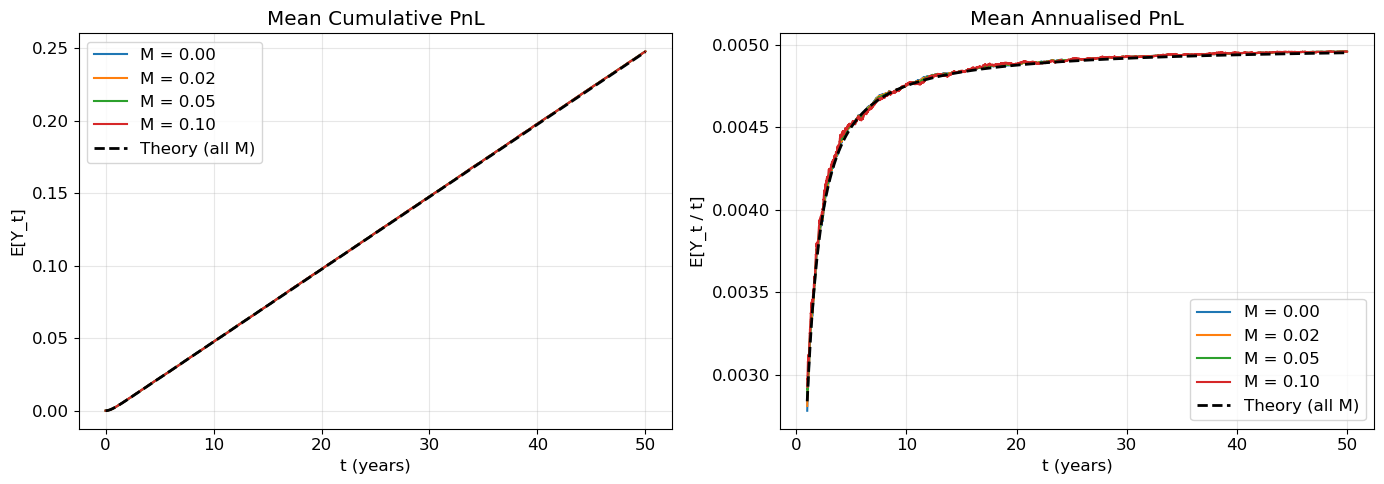
# --- Simulation: expected annualised PnL for different biases M ---
theta, sigma, T, dt = 1.0, 0.10, 50, 1 / 252
n_paths = 5_000
M_values = [0.0, 0.02, 0.05, 0.10]

X = simulate_ou(theta, sigma, T, dt, n_paths)

fig, axes = plt.subplots(1, 2, figsize=(14, 5))

# Left panel: mean cumulative PnL
t_grid = np.arange(X.shape[1]) * dt
theory_mean = 0.5 * (sigma**2 * t_grid - s2(t_grid, theta, sigma))

for M in M_values:
    Y = pnl_paths(X, M, sigma, dt)
    axes[0].plot(t_grid, Y.mean(axis=0), label=f"M = {M:.2f}")

axes[0].plot(t_grid, theory_mean, "k--", lw=2, label="Theory (all M)")
axes[0].set(xlabel="t (years)", ylabel="E[Y_t]", title="Mean Cumulative PnL")
axes[0].legend()

# Right panel: mean annualised PnL (after burn-in)
burn = int(1 / dt)  # skip first year for stability
t_ann = t_grid[burn:]
theory_ann = 0.5 * (sigma**2 - s2(t_ann, theta, sigma) / t_ann)

for M in M_values:
    Y = pnl_paths(X, M, sigma, dt)
    ann = Y[:, burn:] / t_ann
    axes[1].plot(t_ann, ann.mean(axis=0), label=f"M = {M:.2f}")

axes[1].plot(t_ann, theory_ann, "k--", lw=2, label="Theory (all M)")
axes[1].set(xlabel="t (years)", ylabel="E[Y_t / t]", title="Mean Annualised PnL")
axes[1].legend()

print("Observation: All bias levels produce the same expected PnL — the bias washes out.")

plt.tight_layout()plt.show()

Observation: All bias levels produce the same expected PnL — the bias washes out.

2.2 Terminal Variance Increases with Bias

As confirmed in Figure 1, the mean is unaffected, but the dispersion of Y_t grows with |M|. Writing Y_t = \frac{\sigma^2 t}{2} + M X_t - \frac{X_t^2}{2}, the constant drops out of the variance. Using standard Gaussian identities for X \sim \mathcal{N}(0, s^2):

• \operatorname{Var}(X) = s^2,
• \operatorname{Var}(X^2) = 2 s^4 (since \mathbb{E}[X^4] = 3s^4),
• \operatorname{Cov}(X, X^2) = \mathbb{E}[X^3] = 0 (odd moment of a symmetric distribution),

we get

\operatorname{Var}(Y_t) = M^2\, \operatorname{Var}(X_t) + \tfrac{1}{4}\operatorname{Var}(X_t^2)

\boxed{\operatorname{Var}(Y_t) = M^2 s_t^2 + \frac{1}{2}\, s_t^4.}

The first term, M^2 s_t^2, is entirely due to the bias. Even though the bias does not shift the average outcome, it creates a persistent directional long or short tilt roughly M that translates OU fluctuations into PnL variance.

Show simulation code

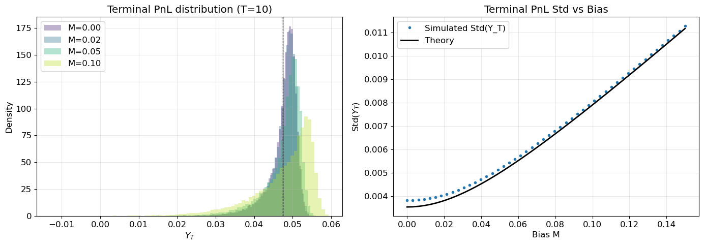
# --- Simulation: terminal PnL distribution for different M ---
theta, sigma, T, dt = 1.0, 0.10, 10, 1 / 252
n_paths = 20_000
X = simulate_ou(theta, sigma, T, dt, n_paths)

fig, axes = plt.subplots(1, 2, figsize=(14, 5))

colors = plt.cm.viridis(np.linspace(0.1, 0.9, len(M_values)))
st2 = s2(T, theta, sigma)

for M, c in zip(M_values, colors):
    Y = pnl_paths(X, M, sigma, dt)
    Y_T = Y[:, -1]

    # Simulated
    axes[0].hist(Y_T, bins=80, density=True, alpha=0.35, color=c, label=f"M={M:.2f}")

    # Theory: mean & std
    mu_th = 0.5 * (sigma**2 * T - st2)
    var_th = M**2 * st2 + 0.5 * st2**2
    axes[0].axvline(mu_th, color="k", ls="--", lw=0.8)

axes[0].set(xlabel="$Y_T$", ylabel="Density", title=f"Terminal PnL distribution (T={T})")
axes[0].legend()

# Right panel: simulated vs theoretical std
M_scan = np.linspace(0, 0.15, 50)
sim_std = []
for M in M_scan:
    Y = pnl_paths(X, M, sigma, dt)
    sim_std.append(Y[:, -1].std())
theory_std = np.sqrt(M_scan**2 * st2 + 0.5 * st2**2)

axes[1].plot(M_scan, sim_std, "o", ms=3, label="Simulated Std(Y_T)")
axes[1].plot(M_scan, theory_std, "k-", lw=2, label="Theory")
axes[1].set(xlabel="Bias M", ylabel="Std($Y_T$)", title="Terminal PnL Std vs Bias")
axes[1].legend()

print(f"Theory std at M=0: {np.sqrt(0.5 * st2**2):.4f},  at M=0.10: {np.sqrt(0.10**2 * st2 + 0.5 * st2**2):.4f}")

plt.tight_layout()plt.show()

Theory std at M=0: 0.0035,  at M=0.10: 0.0079

3 Quadratic Variation

As discussed in Part 1, the terminal variance \operatorname{Var}(Y_t/t) \sim O(1/t^2) shrinks with horizon and understates the volatility experienced along the path. The more relevant risk measure for drawdowns and margin is the quadratic variation of the PnL process.

From the OU dynamics dX_t = -\theta X_t\, dt + \sigma\, dW_t, the PnL differential is

dY_t = -(X_t - M)\, dX_t = \theta X_t(X_t - M)\, dt - \sigma(X_t - M)\, dW_t.

The quadratic variation of Y accumulates only through the martingale part:

d\langle Y \rangle_t = \sigma^2 (X_t - M)^2\, dt.

Taking expectations:

\mathbb{E}[(X_t - M)^2] = \mathbb{E}[X_t^2] - 2M\,\mathbb{E}[X_t] + M^2 = s_t^2 + M^2.

The expected annualised quadratic variation is therefore

\frac{1}{t}\,\mathbb{E}[\langle Y \rangle_t] = \frac{1}{t}\int_0^t \sigma^2(s_u^2 + M^2)\, du = \sigma^2 M^2 + \frac{1}{t}\int_0^t \sigma^2 s_u^2\, du.

Reusing the integral identity from Part 1,

\boxed{ \frac{1}{t}\,\mathbb{E}[\langle Y \rangle_t] = \sigma^2 M^2 + \frac{\sigma^2}{2\theta}\left(\sigma^2 - \frac{s_t^2}{t}\right). }

Compared to the unbiased case, we pick up an additive term \sigma^2 M^2 — a constant “floor” of volatility from the systematic offset position. Figure 2 confirms both results: terminal PnL distributions widen with bias, and the simulated standard deviation matches the theory.

4 Expected Sharpe Ratio

Following the same path-based Sharpe definition as Part 1:

\mathrm{SR}_t := \frac{\mathbb{E}[Y_t / t]}{\sqrt{\mathbb{E}[\langle Y \rangle_t] / t}},

we substitute our expressions for the numerator and denominator. Writing \alpha_t = \sigma^2 - s_t^2/t for brevity:

\boxed{ \mathrm{SR}_t = \frac{\alpha_t / 2}{\sqrt{\sigma^2 M^2 + \frac{\sigma^2}{2\theta}\, \alpha_t}}. }

4.1 Asymptotic Sharpe Ratio

As t \to \infty, s_t^2 \to \sigma^2/(2\theta) and s_t^2/t \to 0, so \alpha_t \to \sigma^2. Hence

\mathrm{SR}_\infty = \frac{\sigma^2/2}{\sqrt{\sigma^2 M^2 + \sigma^4/(2\theta)}} = \frac{\sigma/2}{\sqrt{M^2 + \sigma^2/(2\theta)}}.

This can be written more revealingly as

\boxed{ \mathrm{SR}_\infty = \sqrt{\frac{\theta}{2}} \cdot \frac{1}{\sqrt{1 + \dfrac{2\theta M^2}{\sigma^2}}}. }

The first factor \sqrt{\theta/2} is exactly the unbiased Sharpe from Part 1. The second factor is a penalty that depends on the dimensionless ratio 2\theta M^2/\sigma^2:

• When M = 0, the penalty is 1 and we recover Part 1.
• For fixed M and \sigma, faster mean reversion (\theta large) makes the bias hurt more — the unbiased strategy would have captured cleaner gains, so the same offset position is relatively more costly.
• The penalty is symmetric in M: over-estimating and under-estimating fair value by the same amount are equally harmful.

Show simulation code

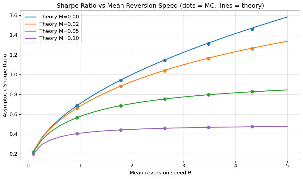
# --- Simulation: Asymptotic Sharpe Ratio vs theta for different M ---

def sr_asymptotic(theta, sigma, M):
    """Closed-form asymptotic SR with bias M."""
    return np.sqrt(theta / 2) / np.sqrt(1 + 2 * theta * M**2 / sigma**2)


theta_range = np.linspace(0.1, 5.0, 30)
sigma = 0.10
T, dt, n_paths = 100, 1 / 252, 1_000
M_values_sr = [0.0, 0.02, 0.05, 0.10]

fig, ax = plt.subplots(figsize=(10, 6))
colors = plt.cm.tab10(np.linspace(0, 0.4, len(M_values_sr)))

for M, c in zip(M_values_sr, colors):
    # Analytical curve
    sr_th = sr_asymptotic(theta_range, sigma, M)
    ax.plot(theta_range, sr_th, "-", color=c, lw=2, label=f"Theory M={M:.2f}")

    # Monte Carlo points (subset of theta values)
    theta_sim = theta_range[::5]
    sr_sim = []
    for th in theta_sim:
        X = simulate_ou(th, sigma, T, dt, n_paths, rng=np.random.default_rng(123))
        Y = pnl_paths(X, M, sigma, dt)
        t_grid = np.arange(X.shape[1]) * dt

        # Annualised mean PnL
        mean_pnl = (Y[:, -1] / T).mean()

        # Annualised QV via discrete approximation
        dX = np.diff(X, axis=1)
        X_mid = X[:, :-1]
        dY_mart = -sigma * (X_mid - M) * (dX + th * X_mid * dt) / sigma  # ≈ -sigma*(X-M)*dW
        # Simpler: compute QV directly as sum of dY^2
        dY = -(X_mid - M) * dX
        qv = np.sum(dY**2, axis=1)
        mean_qv_ann = (qv / T).mean()

        sr_sim.append(mean_pnl / np.sqrt(mean_qv_ann))

    ax.plot(theta_sim, sr_sim, "o", color=c, ms=7, zorder=5)

ax.set(
    xlabel=r"Mean reversion speed $\theta$",
    ylabel="Asymptotic Sharpe Ratio",
    title="Sharpe Ratio vs Mean Reversion Speed (dots = MC, lines = theory)",

)plt.show()

ax.legend(loc="upper left")plt.tight_layout()

Show simulation code

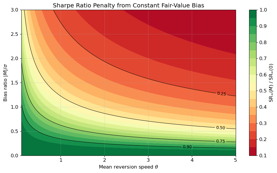
# --- Heatmap: SR penalty factor as function of (theta, M/sigma) ---

theta_grid = np.linspace(0.1, 5.0, 200)
m_ratio_grid = np.linspace(0, 3.0, 200)  # M / sigma
Theta, MR = np.meshgrid(theta_grid, m_ratio_grid)

# Penalty = 1 / sqrt(1 + 2*theta*(M/sigma)^2 * sigma^2/sigma^2) = 1 / sqrt(1 + 2*theta*(M/sigma)^2)
# Wait, let me be precise:
# 2*theta*M^2/sigma^2 = 2*theta*(M/sigma)^2
Penalty = 1.0 / np.sqrt(1 + 2 * Theta * MR**2)

fig, ax = plt.subplots(figsize=(10, 6))
cf = ax.contourf(Theta, MR, Penalty, levels=20, cmap="RdYlGn")
cs = ax.contour(Theta, MR, Penalty, levels=[0.25, 0.5, 0.75, 0.9], colors="k", linewidths=0.8)
ax.clabel(cs, fmt="%.2f", fontsize=10)
plt.colorbar(cf, ax=ax, label=r"$\mathrm{SR}_\infty(M)\;/\;\mathrm{SR}_\infty(0)$")
ax.set(
    xlabel=r"Mean reversion speed $\theta$",
    ylabel=r"Bias ratio $|M|/\sigma$",
    title="Sharpe Ratio Penalty from Constant Fair-Value Bias",

)print("Green = low penalty (bias doesn't hurt much); Red = large penalty.")

plt.tight_layout()plt.show()

Green = low penalty (bias doesn't hurt much); Red = large penalty.

Show simulation code

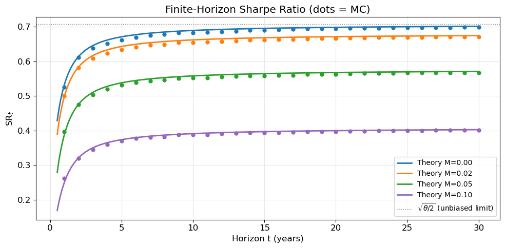
# --- Finite-horizon SR_t vs t for different M ---

theta, sigma = 1.0, 0.10
T, dt, n_paths = 30, 1 / 252, 5_000
X = simulate_ou(theta, sigma, T, dt, n_paths)

fig, ax = plt.subplots(figsize=(10, 5))
eval_years = np.arange(1, int(T) + 1)  # evaluate at integer years

for M, c in zip([0.0, 0.02, 0.05, 0.10], plt.cm.tab10(np.linspace(0, 0.4, 4))):
    # Theory
    t_fine = np.linspace(0.5, T, 500)
    alpha = sigma**2 - s2(t_fine, theta, sigma) / t_fine
    sr_th = (alpha / 2) / np.sqrt(sigma**2 * M**2 + sigma**2 / (2 * theta) * alpha)
    ax.plot(t_fine, sr_th, "-", color=c, lw=2, label=f"Theory M={M:.2f}")

    # Simulated
    sr_sim_pts = []
    for yr in eval_years:
        idx = int(yr / dt)
        if idx >= X.shape[1]:
            break
        Y = pnl_paths(X, M, sigma, dt)
        mean_ann = (Y[:, idx] / yr).mean()
        dX = np.diff(X[:, :idx + 1], axis=1)
        X_mid = X[:, :idx]
        dY = -(X_mid - M) * dX
        qv = np.sum(dY**2, axis=1)
        mean_qv_ann = (qv / yr).mean()
        sr_sim_pts.append(mean_ann / np.sqrt(mean_qv_ann))
    ax.plot(eval_years[:len(sr_sim_pts)], sr_sim_pts, "o", color=c, ms=5)

ax.axhline(np.sqrt(theta / 2), color="gray", ls=":", lw=1, label=r"$\sqrt{\theta/2}$ (unbiased limit)")
ax.set(xlabel="Horizon t (years)", ylabel=r"$\mathrm{SR}_t$",

       title="Finite-Horizon Sharpe Ratio (dots = MC)")plt.show()

ax.legend(loc="lower right", fontsize=10)plt.tight_layout()

5 Discussion

The central finding of this analysis is the invariance of expected PnL to a constant fair-value bias. A persistent error M in the trader’s estimate of fair value does not shift the average outcome (Figure 1), a consequence of the symmetry of X_t about zero: the additional position induced by the bias earns as much on favourable moves as it loses on unfavourable ones. However, this invariance does not extend to risk. The bias creates a systematic offset in the trader’s position — even when there is no true mispricing, the trader holds roughly M units of the asset — adding \sigma^2 M^2 to the annualised quadratic variation and M^2 s_t^2 to the terminal variance (Figure 2).

These two effects combine into a penalty term on the asymptotic Sharpe ratio. The ratio \mathrm{SR}_\infty(M)/\mathrm{SR}_\infty(0) = (1 + 2\theta M^2/\sigma^2)^{-1/2} depends on a single dimensionless quantity: the bias squared, measured in units of the OU stationary standard deviation \sigma/\sqrt{2\theta}. A bias comparable in magnitude to the stationary fluctuation amplitude roughly halves the Sharpe ratio (Figure 3). The penalty is symmetric in M and increases with \theta. Faster mean reversion amplifies the damage, since the unbiased strategy would have captured proportionally larger gains, making the same constant offset relatively more costly (Figure 4). The finite-horizon Sharpe ratio converges monotonically to this asymptotic limit (Figure 5).

6 Extension

The constant-bias model serves as a benchmark against which more realistic estimation structures can be measured. If M is itself a random variable — as it would be when estimated from data — the expected Sharpe integrates over the distribution of M, weighted by estimation uncertainty. A more consequential extension is to allow the bias to be correlated with the price process: Part 1 noted that a fair-value estimate positively correlated with X_t degrades expected PnL through an additional covariance channel, not merely risk. Trailing estimators such as moving averages produce precisely this kind of path-dependent, correlated bias. In the next post we develop the correlated-bias framework and show that it subsumes the constant-M results derived here as a special case.