Expected Performance of a Mean-Reversion Trading Strategy — Part 4
2026-03-03
In Part 1 we derived the asymptotic Sharpe ratio \mathrm{SR}_\infty = \sqrt{\theta/2} of a mean-reversion strategy under the assumption that the mispricing follows an Ornstein-Uhlenbeck process and the trader knows its parameters exactly. Part 2 showed that a constant bias M in the fair-value estimate incurs a multiplicative penalty (1 + \xi^2)^{-1/2}, where \xi = M/s_\infty and s_\infty = \sigma/\sqrt{2\theta} is the stationary mispricing scale. Part 3 extended this to correlated bias, establishing that trailing estimators of fair value degrade both expected PnL and risk.
All three parts treated the OU parameters \theta and \sigma as known. In practice, these must be estimated from a finite calibration sample, and estimation error feeds directly into the trader’s fair-value estimate. In this post we close the loop by quantifying how parameter estimation error affects the realised Sharpe ratio.
We look at the effect of the two estimates separately. The first is the mean estimation error (\hat\mu \neq \mu): the estimated long-run mean acts as a constant bias in the Part 2 sense, with variance \mathrm{Var}(\hat\mu) \approx \sigma^2/(\theta^2 T_{\mathrm{est}}), yielding a penalty (1 + 2/(\theta T_{\mathrm{est}}))^{-1/2} governed entirely by the number of mean-reversion timescales in the calibration window. The second is speed estimation error (\hat\theta \neq \theta): the well-known finite-sample bias in \hat\theta does not alter the pathwise Sharpe ratio of the baseline strategy studied here, but it does create systematic overconfidence when the trader converts \hat\theta into a forecasted Sharpe ratio or a leverage decision, leading to misallocated capital and underestimated drawdowns.
1 Maximum Likelihood Estimation for the OU Process
We work with the same centred OU model as Parts 1–3:
For the trading strategy, X_t represents the mispricing — the deviation from fair value v, with \mu = v denoting the true long-run mean. The trader must estimate the parameter triple (\theta, \mu, \sigma) from a calibration sample of length T_{\mathrm{est}}.
which takes the form of a Gaussian AR(1) model X_{i+1} = a X_i + b + \varepsilon_i with a = e^{-\theta\Delta t} and b = \mu(1-a). Maximum likelihood estimation therefore reduces to OLS regression, and the OU parameters are recovered by inverting:
Three finite-sample difficulties plague this estimator. First, when \theta is small, a \approx 1 and the process resembles a random walk; since the intercept takes the form \mu(1-a), the estimates \hat\mu and \hat\theta become strongly negatively correlated — a slight change in one can be compensated by the other, creating an identification problem. Second, the MLE \hat\theta is upward-biased in finite samples: small-sample variability causes \hat{a} to be pulled below e^{-\theta\Delta t}, which inflates \hat\theta. Third, all three estimators exhibit high variance when \theta T_{\mathrm{est}} is small, reflecting the fact that the process has not completed enough mean-reversion cycles to reveal its parameters reliably.
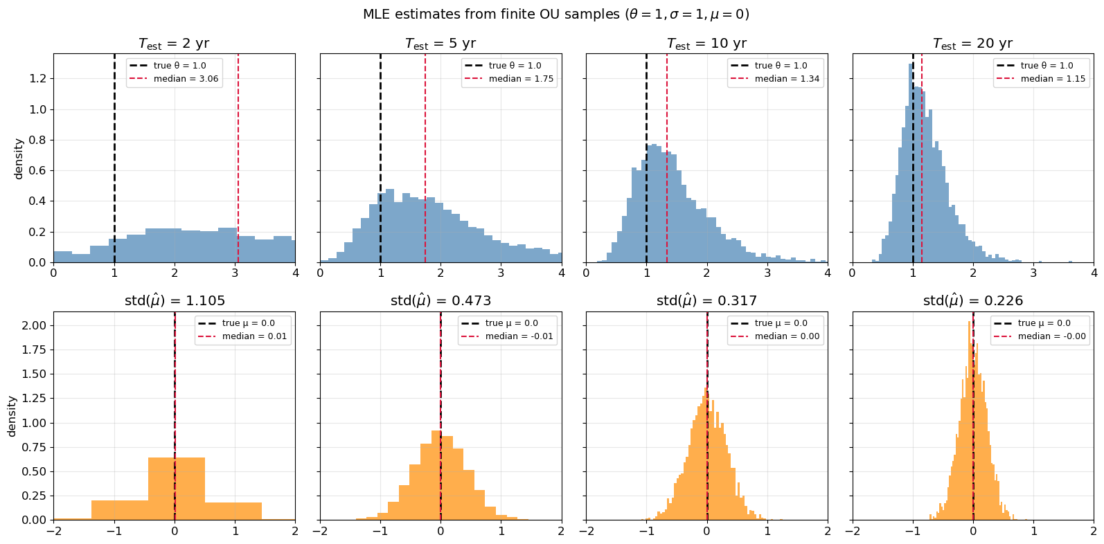
Figure 1 illustrates these effects across calibration windows of 2, 5, 10, and 20 years. The top row shows the distribution of \hat\theta: the median exceeds the true value at short windows and converges from above as more data is observed. The bottom row shows \hat\mu: the distribution is centred at the true mean in all cases, but its standard deviation shrinks only as \sigma/(\theta\sqrt{T_{\mathrm{est}}}), confirming the slow convergence rate inherent to autocorrelated processes.
Figure 1: Finite-sample distributions of MLE estimates \hat\theta (top) and \hat\mu (bottom) for calibration windows of 2, 5, 10, and 20 years (\theta=1, \sigma=1, \mu=0). The upward bias in \hat\theta and the high variance of \hat\mu diminish as the calibration window lengthens.
The trader observes the OU process on a calibration window [0, T_{\mathrm{est}}], estimates (\hat\theta, \hat\mu, \hat\sigma) via MLE, then trades on [T_{\mathrm{est}}, T_{\mathrm{est}} + T_{\mathrm{trade}}] using \hat\mu as the fair-value estimate.
From Part 2, the asymptotic Sharpe ratio when the trader operates with a constant bias M is
Part 2 also demonstrated that expected PnL is unaffected by a constant bias: the degradation acts purely through increased path variance. During the trading window, the estimation error in \hat\mu behaves exactly as a Part 2 constant bias. It is fixed at the moment calibration ends and is independent of the future Brownian increments on [T_{\mathrm{est}}, T_{\mathrm{est}} + T_{\mathrm{trade}}].
2.2 Variance of \hat\mu
For a stationary OU process with mean \mu, the sample mean \bar{X} = \frac{1}{T}\int_0^T X_t\,dt satisfies
This exact expression uses the stationary OU autocovariance. Our simulations below instead start from X_0 = \mu, so the finite-sample covariance kernel differs by a boundary term; the two setups share the same leading asymptotic behaviour, which is the quantity that matters for the long-horizon Sharpe penalty. When \theta T is large, therefore,
Part 3 showed that for a random bias drawn independently of the future price path, the constant-bias formula carries over after averaging over the bias distribution: one replaces \xi^2 by its second moment. Applying that result here with M = \hat\mu therefore yields
The penalty factor \left(1 + 2/(\theta T_{\mathrm{est}})\right)^{-1/2} depends only on the dimensionless product \theta T_{\mathrm{est}} — the number of mean-reversion timescales observed during calibration. To achieve a penalty smaller than 1/\sqrt{2} \approx 0.71, we need \theta T_{\mathrm{est}} > 2, meaning the trader must observe at least two full mean-reversion timescales. Table 1 shows the penalty across a range of calibration lengths.
Table 1: Estimation penalty as a function of calibration length \theta T_{\mathrm{est}}.
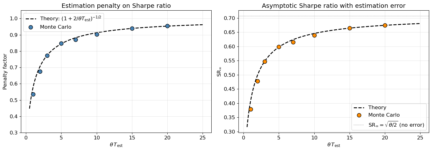
Figure 2: Estimation penalty on Sharpe ratio vs calibration length \theta T_{\mathrm{est}}. Left: penalty factor. Right: absolute SR. Monte Carlo dots closely track the theoretical curve (1 + 2/\theta T_{\mathrm{est}})^{-1/2}.
In Part 3, a correlated bias was shown to degrade expected PnL via -\theta\int_0^t \mathrm{Cov}(M_u, X_u)\,du, not just risk. A natural concern is whether the one-shot estimator \hat\mu — computed from the calibration window — introduces this additional penalty.
Asymptotically, it does not. Note that X_t for t > T_{\mathrm{est}} depends on the calibration window only through X_{T_{\mathrm{est}}}. Since \hat\mu is a function of \{X_s : s \leq T_{\mathrm{est}}\}, the covariance decays exponentially as the trading window progresses:
so the quadratic-variation correction is transient for the same reason. For one-shot estimation, the asymptotic Sharpe penalty therefore comes entirely from the Part 2 variance channel: \hat\mu acts as a random constant bias with \mathbb{E}[\hat\mu^2] \approx \sigma^2/(\theta^2 T_{\mathrm{est}}), yielding the clean formula (1 + 2/(\theta T_{\mathrm{est}}))^{-1/2}. Figure 2 confirms this result with Monte Carlo simulation.
4 Rolling Estimation
In practice, traders do not estimate \hat\mu once and trade indefinitely. In the simplest adaptive setting, they re-estimate continuously using a rolling window of length W. At each time t, the fair-value estimate is the trailing sample mean
M_t = \frac{1}{W}\int_{t-W}^{t} X_s\,ds,
which is a simple moving average (SMA), a trailing estimator of the kind analysed in Part 3. The weighting kernel w(s) = \mathbf{1}_{[0,W]}(s)/W is non-negative and integrates to one, so Part 3’s general theorem guarantees \mathrm{Cov}(M_t, X_t) > 0 at all times. Rolling re-estimation therefore creates the persistent correlated-bias penalty that the one-shot estimator avoids.
For a stationary OU process, the covariance between the rolling estimate and the current mispricing is available in closed form:
Equivalently, the rolling penalty relative to the Part 1 benchmark is
P_{\mathrm{SMA}}(a) = \frac{\mathrm{SR}^{\mathrm{SMA}}_\infty}{\sqrt{\theta/2}} = \frac{A(a)}{\sqrt{2B(a)}}, \qquad a = \theta W
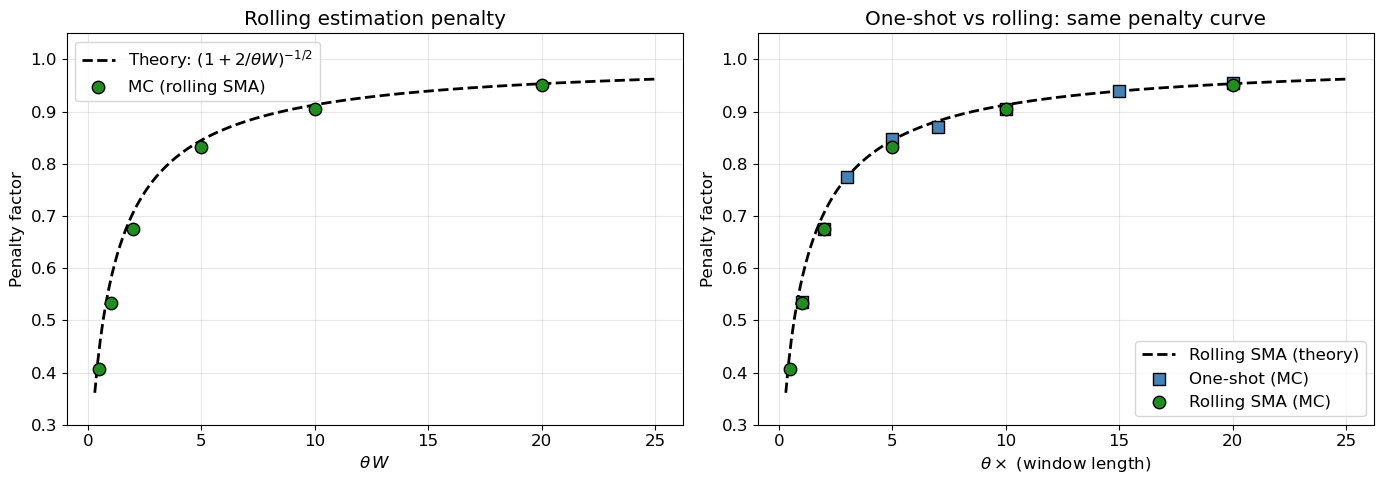
This exact SMA penalty depends only on the dimensionless window length \theta W, just as the one-shot penalty depends only on \theta T_{\mathrm{est}}. The two are not algebraically identical, however: the EMA-based shortcut (1 + 2/(\theta W))^{-1/2} captures the right large-window scaling, but the exact SMA penalty is slightly lower for short windows. That distinction is summarised in Table 2 and confirmed numerically in Figure 3.
Table 2: Penalty source comparison for one-shot vs rolling estimation.
Method
Penalty
Source
One-shot (calibrate then trade)
(1 + 2/(\theta T_{\mathrm{est}}))^{-1/2}
Part 2 variance channel only
Rolling SMA window W
P_{\mathrm{SMA}}(\theta W)
Part 3 covariance channel plus extra path risk
For one-shot estimation, only the Part 2 variance-channel penalty survives at long horizons (the covariance channel washes out), whereas the rolling estimator adds a permanent Part 3 covariance penalty — a structural cost of continuous re-estimation.
Show simulation code
# --- Rolling estimation: SMA bias simulation ---theta_true, sigma_true =1.0, 1.0dt =1/252T =50# total simulation lengthn_paths =2000W_values = [0.5, 1, 2, 5, 10, 20]def sma_penalty_exact(theta, W): a = theta * np.asarray(W, dtype=float) one_minus_exp =1- np.exp(-a) A =1- one_minus_exp / a B =0.5- one_minus_exp / a + (a - one_minus_exp) / a**2return A / np.sqrt(2* B)sr_rolling_mc = []for W in W_values: W_steps =int(W / dt) X = simulate_ou(theta_true, sigma_true, T, dt, n_paths, rng=np.random.default_rng(123))# Compute rolling SMA bias: M_t = (1/W) * integral_{t-W}^{t} X_s ds cumX = np.cumsum(X, axis=1) * dt M = np.zeros_like(X)for k inrange(W_steps, X.shape[1]): M[:, k] = (cumX[:, k] - cumX[:, k - W_steps]) / W# Only measure SR after the window is fully populated burn = W_steps +int(5/ dt)if burn >= X.shape[1] -int(5/ dt): burn = W_steps X_eval = X[:, burn:] M_eval = M[:, burn:] T_eval = (X_eval.shape[1] -1) * dt# SR = mean(annualised PnL) / sqrt(mean(annualised QV_Y)) Y = pnl_paths(X_eval, M_eval, dt) mean_pnl = np.mean(Y[:, -1] / T_eval) dX_eval = np.diff(X_eval, axis=1) dY =-(X_eval[:, :-1] - M_eval[:, :-1]) * dX_eval qvY = np.sum(dY**2, axis=1) mean_qvY = np.mean(qvY / T_eval) sr_rolling_mc.append(mean_pnl / np.sqrt(mean_qvY))sr_rolling_mc = np.array(sr_rolling_mc)# --- Plot: rolling SR vs window ---fig, axes = plt.subplots(1, 2, figsize=(14, 5))# Left: exact rolling-SMA penalty vs theta*WW_fine = np.linspace(0.3, 25, 200)penalty_sma_theory = sma_penalty_exact(theta_true, W_fine)axes[0].plot(theta_true * W_fine, penalty_sma_theory, 'k-', lw=2, label=r'Exact SMA theory')penalty_rolling = sr_rolling_mc / np.sqrt(theta_true /2)axes[0].scatter(theta_true * np.array(W_values), penalty_rolling, s=80, c='forestgreen', zorder=5, edgecolors='black', label='MC (rolling SMA)')axes[0].set_xlabel(r'$\theta \, W$')axes[0].set_ylabel('Penalty factor')axes[0].set_title('Rolling estimation penalty')axes[0].legend()axes[0].set_ylim(0.2, 1.05)# Right: compare one-shot and rolling on the same dimensionless scaleone_shot_theory =1/ np.sqrt(1+2/ W_fine)axes[1].plot(W_fine, one_shot_theory, 'k--', lw=2, label='One-shot theory')axes[1].plot(W_fine, penalty_sma_theory, color='forestgreen', lw=2, label='Rolling SMA theory')axes[1].scatter(theta_true * T_est_grid, sr_mc / np.sqrt(theta_true /2), s=80, c='steelblue', zorder=5, edgecolors='black', marker='s', label='One-shot (MC)')axes[1].scatter(theta_true * np.array(W_values), penalty_rolling, s=80, c='forestgreen', zorder=5, edgecolors='black', marker='o', label='Rolling SMA (MC)')axes[1].set_xlabel(r'Dimensionless history length ($\theta T_{\mathrm{est}}$ or $\theta W$)')axes[1].set_ylabel('Penalty factor')axes[1].set_title('One-shot vs rolling: same scale, different curves')axes[1].legend()axes[1].set_ylim(0.2, 1.05)fig.tight_layout()plt.show()# Summary table as Markdownrows = []for W, sr inzip(W_values, sr_rolling_mc): th_penalty = sma_penalty_exact(theta_true, W) rows.append(f"| {W:.1f} | {theta_true * W:.1f} | {sr:.4f} | "f"{sr / np.sqrt(theta_true /2):.3f} | {th_penalty:.3f} |" )table ="\n".join([r"|$W$(yr)|$\theta W$| SR (MC)| Penalty (MC)| Penalty (exact SMA theory)|","|:---:|:---:|:---:|:---:|:---:|",*rows,])display(Markdown(table))
Figure 3: Rolling SMA penalty vs window length. Left: Monte Carlo penalty factor for the rolling SMA against the exact stationary SMA theory. Right: one-shot and rolling penalties compared on the common scale variable, showing similar scaling but different exact curves.
It is well known that the MLE overestimates \theta in finite samples: the median \hat\theta exceeds the true value, as shown in Figure 1. A natural question is whether this bias can degrade the realised Sharpe ratio in practice.
For the baseline strategy studied throughout this series, it does not enter the pathwise Sharpe ratio directly. The trading rule uses only the estimated fair value, with PnL
dY_t = -(X_t - \hat\mu)\,dX_t,
so replacing \theta by \hat\theta does not change the signal itself. In that sense the realised Sharpe ratio of the base strategy is invariant to speed-estimation error. A \theta-dependent sizing rule would be a different strategy and would generally reintroduce direct dependence on \hat\theta.
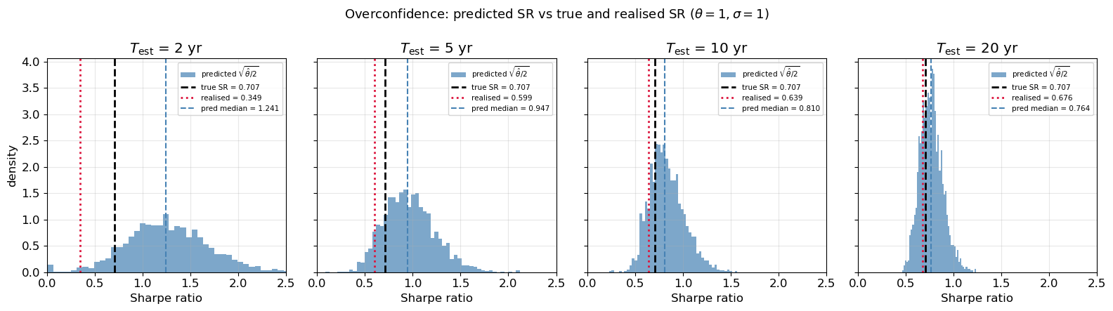
However, a trader who computes the predicted Sharpe ratio \mathrm{SR}_\infty = \sqrt{\hat\theta/2} will arrive at a systematic overestimate, since \hat\theta is upward-biased. The resulting overconfidence distorts capital allocation: more capital or higher leverage is deployed than the strategy’s actual risk-reward profile warrants. Risk budgets calibrated to the inflated SR become too tight, raising the probability of premature stop-outs during normal drawdowns. In a multi-strategy portfolio, the allocation problem is compounded: the strategy with the shortest calibration window appears most attractive precisely because its \hat\theta is the most inflated. Figure 4 quantifies this gap between predicted and realised SR for calibration windows of 2-20 years.
Figure 4: Distribution of predicted SR \sqrt{\hat\theta/2} vs true and realised SR for calibration lengths of 2, 5, 10, and 20 years. The median prediction systematically exceeds realised SR, with the gap narrowing as the calibration window lengthens.
The central result of this post is a closed-form expression for the one-shot estimation penalty on Sharpe ratio. When a trader calibrates the OU process on a window of length T_{\mathrm{est}} and then trades with the estimated fair value, the asymptotic Sharpe ratio is \mathrm{SR}_\infty = \sqrt{\theta/2}\,(1 + 2/(\theta T_{\mathrm{est}}))^{-1/2}, as confirmed by Monte Carlo in Figure 2 and tabulated in Table 1. The penalty depends entirely on \theta T_{\mathrm{est}}, the number of mean-reversion timescales observed during calibration. Slow mean reversion (small \theta) therefore demands proportionally longer calibration to achieve the same penalty level.
A key structural distinction separates one-shot estimation from rolling re-estimation. The one-shot estimator \hat\mu is fixed at the end of calibration and is independent of subsequent Brownian increments, so it enters as a Part 2 constant bias whose correlation with the trading-window process decays exponentially. For long trading horizons, the Part 3 covariance channel washes out entirely and only the variance penalty remains. The rolling estimator, by contrast, continuously updates \hat\mu using a trailing window of length W, creating a permanent positive correlation between the bias and the mispricing. Its exact SMA penalty is a different function of the dimensionless window length \theta W, even though both one-shot and rolling estimation are governed by the same basic principle: too little effective history relative to the mean-reversion timescale degrades risk-adjusted performance.
Taken together, Parts 1-4 give a clean decomposition of where Sharpe-ratio losses come from in this simple mean-reversion setting. Perfect information delivers the benchmark \sqrt{\theta/2}. A constant bias leaves expected PnL intact but raises path risk. A trailing estimator adds a covariance penalty on top of that. Finite-sample parameter estimation then links these abstract bias channels to a concrete statistical object: the amount of usable calibration history measured in OU timescales.