Expected Performance of a Mean-Reversion Trading Strategy

Parts 1–5 of this series analysed the performance of a mean-reversion strategy under a single, powerful simplification: the asset’s fair value v was held constant. Every price change was therefore a change in mispricing, and the trader’s only challenge was to estimate the level v from noisy data.

In practice, fair value itself moves — driven by fundamentals, regime shifts, or slow-moving macroeconomic factors. When it does, the price signal p_t = v_t + X_t conflates two distinct sources of variation: fast mean-reverting mispricing X_t (which the strategy profits from) and slow fair-value drift v_t (which it does not). A trailing estimator like the EMA cannot distinguish the two, and this creates a new penalty channel that has no analogue in Parts 1–5.

This post develops the two-scale OU model — mispricing reverts fast, fair value reverts slowly — and derives the modified Sharpe ratio formulas. The key results are:

1 The Two-Scale OU Model

We generalise the Parts 1–5 framework by allowing fair value to follow its own mean-reverting process on a slow timescale:

dv_t = -\theta_v\,(v_t - \bar{v})\, dt + \sigma_v\, dW_t^v, \qquad dX_t = -\theta\, X_t\, dt + \sigma\, dW_t,

where W^v \perp W, \theta_v > 0 is the fair-value mean-reversion speed, \bar{v} is the long-run fair value, and \sigma_v > 0 is the fair-value volatility. The mispricing X_t = p_t - v_t follows the same OU process as before. Typically \theta_v \ll \theta: fair value moves slowly relative to mispricing.

dp_t = dv_t + dX_t = -\theta_v(v_t - \bar{v})\, dt - \theta X_t\, dt + \sigma_v\, dW_t^v + \sigma\, dW_t.

The trader’s PnL from position -\tilde{X}_t = -(X_t - M_t) now splits into two terms:

dY_t = -(X_t - M_t)\, dp_t = \underbrace{-(X_t - M_t)\, dX_t}_{\text{mean-reversion PnL (Parts 1–5)}} \;\underbrace{-\; (X_t - M_t)\, dv_t}_{\text{fair-value drift exposure (new)}}.

The first term is the familiar mean-reversion profit. The second term is new: the trader’s position is exposed to fair-value movements. Since the EMA bias M_t is correlated with v_t (through the lagged tracking), this second term has nonzero expectation and creates an additional penalty.

Three dimensionless parameters govern the new model: the timescale ratio \theta_v/\theta, the noise ratio \rho = \sigma_v/\sigma, and the EMA bandwidth \lambda/\theta.

2 Irreducible Penalty from Fair-Value Noise

Even if the trader has perfect information — observing X_t directly and trading with M = 0 — the fair-value noise imposes an irreducible penalty. With position -X_t:

The expected PnL rate is unaffected: \mathbb{E}[-X_t\, dv_t/dt] = -\theta_v\,\mathbb{E}[X_t\, u_t] = 0 because X_t and u_t = v_t - \bar{v} are driven by independent Brownian motions. The expected PnL remains \sigma^2/2.

The asymptotic QV rate is (\sigma^2 + \sigma_v^2)\, s_\infty^2 where s_\infty^2 = \sigma^2/(2\theta). Therefore:

\boxed{\mathrm{SR}_\infty^{\text{perfect}} = \sqrt{\frac{\theta}{2}} \cdot \frac{1}{\sqrt{1 + \sigma_v^2/\sigma^2}}.}

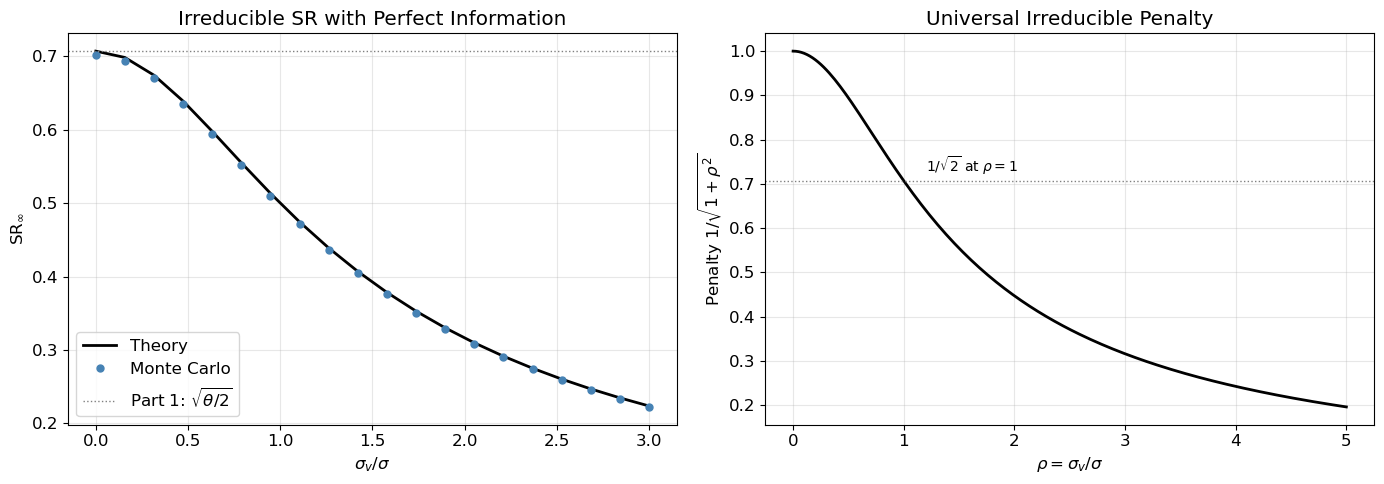
This has the same functional form as Part 2’s bias penalty, but here the penalty is irreducible: it cannot be mitigated by better estimation, since it arises from the trader’s position being exposed to the orthogonal fair-value noise. The ratio \rho = \sigma_v/\sigma plays the role of a signal-to-noise ratio: when fair-value volatility dominates (\rho \gg 1), most of the price variation is uninformative, and the Sharpe ratio collapses.

Figure 1 verifies this formula and shows the penalty surface over (\theta_v/\theta, \sigma_v/\sigma). Note that the irreducible penalty depends only on \rho, not on \theta_v — the speed at which fair value reverts is irrelevant when information is perfect.

Show simulation code

# --- Experiment 1: Irreducible fair-value penalty ---
theta, sigma = 1.0, 0.10
theta_v = 0.2
T, dt, n_paths = 100, 1 / 252, 3_000

rho_scan = np.linspace(0, 3.0, 20)
sr_theory_perf = [sr_perfect_info(theta, sigma, r * sigma) for r in rho_scan]
sr_mc_perf = []

for rho in rho_scan:
    sv = rho * sigma
    sim_rng = np.random.default_rng(42)
    u, X, _ = simulate_two_scale_ou(theta, theta_v, sigma, sv, 0.0, T, dt, n_paths, rng=sim_rng)
    # Perfect info: M = 0, so X_tilde = X
    M_zero = np.zeros_like(X)
    sr = compute_sr_mc(u, X, M_zero, sigma, sv, dt, T)
    sr_mc_perf.append(sr)

fig, axes = plt.subplots(1, 2, figsize=(14, 5))

axes[0].plot(rho_scan, sr_theory_perf, 'k-', lw=2, label='Theory')
axes[0].plot(rho_scan, sr_mc_perf, 'o', ms=5, color='steelblue', label='Monte Carlo')
axes[0].axhline(np.sqrt(theta / 2), color='gray', ls=':', lw=1,
                label=r'Part 1: $\sqrt{\theta/2}$')
axes[0].set_xlabel(r'$\sigma_v / \sigma$')
axes[0].set_ylabel(r'$\mathrm{SR}_\infty$')
axes[0].set_title('Irreducible SR with Perfect Information')
axes[0].legend()

# Right: universal penalty curve
rho_fine = np.linspace(0, 5, 200)
penalty = 1 / np.sqrt(1 + rho_fine**2)
axes[1].plot(rho_fine, penalty, 'k-', lw=2)
axes[1].axhline(1 / np.sqrt(2), color='gray', ls=':', lw=1)
axes[1].text(1.2, 1 / np.sqrt(2) + 0.02, r'$1/\sqrt{2}$ at $\rho=1$', fontsize=10)
axes[1].set_xlabel(r'$\rho = \sigma_v / \sigma$')
axes[1].set_ylabel(r'Penalty $1/\sqrt{1+\rho^2}$')
axes[1].set_title('Universal Irreducible Penalty')

plt.tight_layout()
plt.show()

Figure 1: Irreducible penalty from fair-value noise. Left: SR vs \sigma_v/\sigma with perfect information (M=0), comparing theory to Monte Carlo. Right: the penalty factor 1/\sqrt{1+\rho^2} as a universal curve.

3 EMA Estimator Under Mean-Reverting Fair Value

3.1 Bias dynamics

The EMA tracks p_t: d\tilde{v}_t = \lambda(p_t - \tilde{v}_t)\, dt. Since p_t = \bar{v} + u_t + X_t and \tilde{v}_t = \bar{v} + u_t + X_t - \tilde{X}_t = v_t + M_t, the bias M_t = \tilde{v}_t - v_t satisfies:

The first term is new: the EMA must absorb fair-value drift. The joint system (u_t, X_t, M_t) has drift matrix

A = \begin{pmatrix} -\theta_v & 0 & 0 \\ 0 & -\theta & 0 \\ \theta_v & \lambda & -\lambda \end{pmatrix}

and diffusion covariance Q = BB^\top where B = \text{diag}(\sigma_v, \sigma, -\sigma_v).

3.2 Stationary moments

The Lyapunov equation A\Sigma + \Sigma A^\top + Q = 0 yields six closed-form entries. The first three are unchanged from simpler models:

\Sigma_{uu} = \frac{\sigma_v^2}{2\theta_v}, \qquad \Sigma_{uX} = 0, \qquad \Sigma_{XX} = \frac{\sigma^2}{2\theta}.

\Sigma_{uM} = -\frac{\sigma_v^2}{2(\theta_v + \lambda)}, \qquad \Sigma_{XM} = \frac{\lambda\sigma^2}{2\theta(\theta + \lambda)}, \qquad \Sigma_{MM} = \frac{\lambda\sigma^2}{2\theta(\theta + \lambda)} + \frac{\sigma_v^2}{2(\theta_v + \lambda)}.

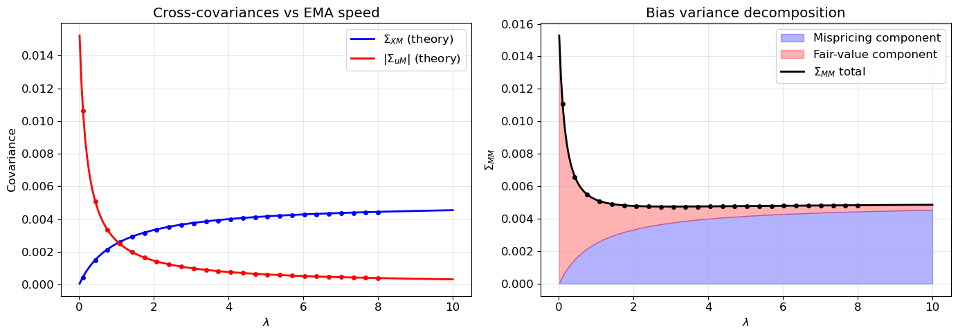
The cross-covariance \Sigma_{XM} is identical to Part 3 — the EMA’s interaction with mispricing is unaffected by fair-value dynamics (because u and X are independent). The bias variance \Sigma_{MM} decomposes additively into the mispricing tracking error \lambda\sigma^2/(2\theta(\theta+\lambda)) from Part 3 and a new fair-value tracking error \sigma_v^2/(2(\theta_v + \lambda)).

The covariance \Sigma_{uM} < 0 has a natural interpretation: when v_t > \bar{v} (i.e., u > 0), the EMA lags behind, so \hat{v} < v and M < 0.

3.3 Variance of perceived mispricing

\operatorname{Var}(\tilde{X}) = \operatorname{Var}(X - M) = \Sigma_{XX} - 2\Sigma_{XM} + \Sigma_{MM} = \frac{\sigma^2}{2(\theta + \lambda)} + \frac{\sigma_v^2}{2(\theta_v + \lambda)}.

This is a clean additive decomposition: each noise source contributes its variance divided by twice the sum of its own reversion speed and the EMA bandwidth. Figure 2 confirms these stationary moments via Monte Carlo.

Show simulation code

theta, sigma, theta_v, sigma_v = 1.0, 0.10, 0.2, 0.08
T, dt, n_paths = 100, 1 / 252, 5_000
lam_scan = np.linspace(0.1, 8.0, 25)

# Theory
lam_fine = np.linspace(0.01, 10.0, 200)
SigXM_th = lam_fine * sigma**2 / (2 * theta * (theta + lam_fine))
SiguM_th = -sigma_v**2 / (2 * (theta_v + lam_fine))
SigMM_th = lam_fine * sigma**2 / (2 * theta * (theta + lam_fine)) + sigma_v**2 / (2 * (theta_v + lam_fine))

# MC
SigXM_mc, SiguM_mc, SigMM_mc = [], [], []
for lam in lam_scan:
    sim_rng = np.random.default_rng(42)
    u, X, M = simulate_two_scale_ou(theta, theta_v, sigma, sigma_v, lam, T, dt, n_paths, rng=sim_rng)
    half = X.shape[1] // 2
    SigXM_mc.append(np.mean(X[:, half:] * M[:, half:]))
    SiguM_mc.append(np.mean(u[:, half:] * M[:, half:]))
    SigMM_mc.append(np.mean(M[:, half:]**2))

fig, axes = plt.subplots(1, 2, figsize=(14, 5))

axes[0].plot(lam_fine, SigXM_th, 'b-', lw=2, label=r'$\Sigma_{XM}$ (theory)')
axes[0].plot(lam_scan, SigXM_mc, 'bo', ms=4)
axes[0].plot(lam_fine, np.abs(SiguM_th), 'r-', lw=2, label=r'$|\Sigma_{uM}|$ (theory)')
axes[0].plot(lam_scan, np.abs(SiguM_mc), 'ro', ms=4)
axes[0].set_xlabel(r'$\lambda$')
axes[0].set_ylabel('Covariance')
axes[0].set_title('Cross-covariances vs EMA speed')
axes[0].legend()

# Components of Sigma_MM
comp_X = lam_fine * sigma**2 / (2 * theta * (theta + lam_fine))
comp_v = sigma_v**2 / (2 * (theta_v + lam_fine))
axes[1].fill_between(lam_fine, 0, comp_X, alpha=0.3, color='blue', label='Mispricing component')
axes[1].fill_between(lam_fine, comp_X, comp_X + comp_v, alpha=0.3, color='red', label='Fair-value component')
axes[1].plot(lam_fine, SigMM_th, 'k-', lw=2, label=r'$\Sigma_{MM}$ total')
axes[1].plot(lam_scan, SigMM_mc, 'ko', ms=4)
axes[1].set_xlabel(r'$\lambda$')
axes[1].set_ylabel(r'$\Sigma_{MM}$')
axes[1].set_title('Bias variance decomposition')
axes[1].legend()

plt.tight_layout()
plt.show()

Figure 2: Stationary moments of the two-scale OU + EMA system vs \lambda. Theory (lines) matches Monte Carlo (dots). Left: \Sigma_{XM} (unchanged from Part 3) and |\Sigma_{uM}| (new, from fair-value tracking). Right: \Sigma_{MM} decomposes into mispricing and fair-value components.

4 Modified Sharpe Ratio

4.1 Expected PnL rate

\boxed{\mathbb{E}[\text{PnL rate}] = \frac{\theta\sigma^2}{2(\theta + \lambda)} - \frac{\theta_v\sigma_v^2}{2(\theta_v + \lambda)}.}

The two terms have a striking parallel structure: each is the product of the reversion speed, the noise variance, and an EMA penalty factor. The first is profit (from correctly trading mispricing); the second is loss (from mistakenly trading fair-value movements as if they were mispricing). When the EMA is slow (\lambda small), the first term is large but the second is also large: the trader profits from mispricing but loses on fair-value tracking. When the EMA is fast (\lambda large), both terms shrink.

4.2 Viability condition

Equivalently, \theta/\theta_v > \rho^2. The strategy is viable only when the mispricing signal (\theta\sigma^2, reflecting both the speed and magnitude of mean reversion) exceeds the fair-value noise (\theta_v\sigma_v^2). This is the two-scale analogue of the signal-to-noise condition.

4.3 Quadratic variation and Sharpe ratio

\text{QV rate} = (\sigma^2 + \sigma_v^2)\left[\frac{\sigma^2}{2(\theta + \lambda)} + \frac{\sigma_v^2}{2(\theta_v + \lambda)}\right].

\boxed{\mathrm{SR}_\infty(\lambda) = \frac{\dfrac{\theta\sigma^2}{2(\theta+\lambda)} - \dfrac{\theta_v\sigma_v^2}{2(\theta_v+\lambda)}}{\sqrt{(\sigma^2 + \sigma_v^2)\left[\dfrac{\sigma^2}{2(\theta+\lambda)} + \dfrac{\sigma_v^2}{2(\theta_v+\lambda)}\right]}}.}

Setting \sigma_v = 0 recovers the Part 3 result \theta/\sqrt{2(\theta + \lambda)}.

4.4 Optimal EMA speed

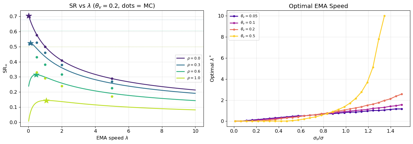
The optimal \lambda^* balances two opposing forces: slower EMA preserves mispricing profit but incurs large fair-value tracking losses; faster EMA reduces fair-value losses but also destroys the mispricing signal. The optimal \lambda^* satisfies a nonlinear equation and must be found numerically in general; Figure 3 shows the SR as a function of \lambda for several parameter configurations.

Show simulation code

theta, sigma = 1.0, 0.10
T, dt, n_paths = 100, 1 / 252, 3_000

fig, axes = plt.subplots(1, 2, figsize=(14, 5))

# Left: SR(lambda) for several sigma_v values
theta_v_fixed = 0.2
sigma_v_ratios = [0.0, 0.3, 0.6, 1.0]
lam_range = np.linspace(0.01, 10.0, 200)
colors = plt.cm.viridis(np.linspace(0.1, 0.9, len(sigma_v_ratios)))

for rho, c in zip(sigma_v_ratios, colors):
    sv = rho * sigma
    sr_th = np.array([sr_ema_two_scale(theta, theta_v_fixed, sigma, sv, l) for l in lam_range])
    axes[0].plot(lam_range, sr_th, color=c, lw=2, label=f'$\\rho = {rho}$')

    # Optimal lambda
    if sr_th.max() > 0:
        best_idx = np.argmax(sr_th)
        axes[0].plot(lam_range[best_idx], sr_th[best_idx], '*', ms=15, color=c, zorder=5)

    # MC verification at a few points
    lam_mc_pts = [0.5, 1.0, 2.0, 5.0]
    for lam_pt in lam_mc_pts:
        sim_rng = np.random.default_rng(42)
        u, X, M = simulate_two_scale_ou(theta, theta_v_fixed, sigma, sv, lam_pt, T, dt, n_paths, rng=sim_rng)
        sr_mc = compute_sr_mc(u, X, M, sigma, sv, dt, T)
        axes[0].plot(lam_pt, sr_mc, 'o', ms=5, color=c, zorder=5)

    # Irreducible SR
    if rho > 0:
        sr_irr = sr_perfect_info(theta, sigma, sv)
        axes[0].axhline(sr_irr, color=c, ls=':', lw=1, alpha=0.5)

axes[0].set_xlabel(r'EMA speed $\lambda$')
axes[0].set_ylabel(r'$\mathrm{SR}_\infty$')
axes[0].set_title(f'SR vs $\\lambda$ ($\\theta_v = {theta_v_fixed}$, dots = MC)')
axes[0].legend(fontsize=9)

# Right: optimal lambda* vs rho for several theta_v
theta_v_values = [0.05, 0.1, 0.2, 0.5]
rho_scan_opt = np.linspace(0.01, 1.5, 30)
tv_colors = plt.cm.plasma(np.linspace(0.1, 0.9, len(theta_v_values)))

for tv, tc in zip(theta_v_values, tv_colors):
    opt_lams = []
    for rho in rho_scan_opt:
        sv = rho * sigma
        sr_curve = np.array([sr_ema_two_scale(theta, tv, sigma, sv, l) for l in lam_range])
        if sr_curve.max() > 0:
            opt_lams.append(lam_range[np.argmax(sr_curve)])
        else:
            opt_lams.append(np.nan)
    axes[1].plot(rho_scan_opt, opt_lams, 'o-', ms=4, lw=2, color=tc, label=f'$\\theta_v = {tv}$')

axes[1].set_xlabel(r'$\sigma_v / \sigma$')
axes[1].set_ylabel(r'Optimal $\lambda^*$')
axes[1].set_title('Optimal EMA Speed')
axes[1].legend(fontsize=9)

plt.tight_layout()
plt.show()

Figure 3: Sharpe ratio vs EMA speed under two-scale OU model. Left: SR(\lambda) for several \sigma_v values with \theta_v = 0.2. Stars mark optimal \lambda^*. Dashed lines show irreducible SR. Right: optimal \lambda^* vs \sigma_v/\sigma for several \theta_v values.

5 Kalman Filter Preview

The EMA is a one-parameter filter that treats p_t as a single signal. The Kalman-Bucy filter for the two-scale OU system does better by exploiting the known dynamics: it separately tracks v_t and X_t using the full state-space structure.

In state-space form, the state (u_t, X_t)^\top has dynamics dx = Fx\, dt + G\, dW and the observation is dp_t = Cx\, dt + H\, dW (same Brownian motions, creating correlated state and observation noise). The steady-state error covariance P_\infty satisfies the continuous-time algebraic Riccati equation, and the Kalman gain K provides the optimal linear filter.

The KF produces separate estimates \hat{u}_t and \hat{X}_t with gains that automatically balance the two timescales — fast mean reversion in X vs slow reversion in u. The residual estimation error \text{Var}(X_t - \hat{X}_t) is smaller than the EMA’s error \text{Var}(X_t - \tilde{X}_t + M_t) because the KF does not conflate the two sources of variation.

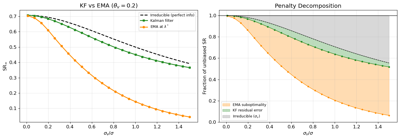
Figure 4 shows the SR achieved by the Kalman filter vs the EMA at optimal \lambda^*. The gap represents the cost of using a naive one-parameter filter rather than the optimal two-parameter filter.

Show simulation code

theta, sigma = 1.0, 0.10
theta_v = 0.2
rho_scan_kf = np.linspace(0.01, 1.5, 25)
lam_range_kf = np.linspace(0.01, 15.0, 300)

sr_irr_list, sr_kf_list, sr_ema_opt_list = [], [], []

for rho in rho_scan_kf:
    sv = rho * sigma

    # Irreducible
    sr_irr_list.append(sr_perfect_info(theta, sigma, sv))

    # KF: solve Riccati, get residual error variance for X
    P, K = kalman_steady_state(theta, theta_v, sigma, sv)
    # P[1,1] is Var(X - X_hat), P[0,0] is Var(u - u_hat)
    var_X_err = P[1, 1]
    # The KF estimate of X has error M_kf with Var = var_X_err
    # And Cov(M_kf, X) = ? For the KF, the error is uncorrelated with the estimate (orthogonality)
    # So the SR formula: E[PnL] uses the covariance structure.
    # For a proper SR, we'd need the full covariance of the KF state.
    # Approximation: treat KF error as independent bias with variance P[1,1]
    # SR_kf ≈ sqrt(theta/2) / sqrt(1 + P[1,1]/s_inf^2) / sqrt(1 + sigma_v^2/sigma^2)
    # But this double-counts. The correct formula:
    # E[PnL] = theta * (s_inf^2 - Cov(X, M_kf))  (mispricing part, M_kf is KF error)
    # For the KF, the innovation is orthogonal to the estimate, so Cov(X, X-X_hat) = Var(X-X_hat)
    # Therefore Cov(X_hat, X) = Var(X) - Var(X-X_hat) = s_inf^2 - P[1,1]
    # And Cov(M_kf, X) = Cov(X - X_hat, X) = P[1,1]
    # So E[PnL from MR] = theta*(s_inf^2 - P[1,1])
    s_inf2 = sigma**2 / (2 * theta)
    # Fair-value part: E[(X - M_kf)(-theta_v u)] = -theta_v Cov(X_hat, u)
    # Since X_hat = X - (X-X_hat), Cov(X_hat, u) = Cov(X, u) - Cov(X-X_hat, u) = 0 - P[0,1]
    # So fair-value loss = -theta_v * (0 - (-P[0,1])) = -theta_v * P[0,1]  ...need sign care
    # Actually: position is -(X_hat), PnL from dv: -X_hat * dv
    # E[-X_hat * (-theta_v u)] = theta_v Cov(X_hat, u) = theta_v * (Cov(X,u) - P[0,1])
    # = theta_v * (0 - P[0,1]) = -theta_v * P[0,1]

    # With P from Riccati:
    e_pnl_kf = theta * (s_inf2 - P[1, 1]) - theta_v * P[0, 1]

    # QV: (sigma^2 + sigma_v^2) * E[X_hat^2]
    # E[X_hat^2] = Var(X_hat) = s_inf^2 - P[1,1]  (X_hat = X - error, Var(X_hat) = Var(X) - Var(error))
    var_Xhat = s_inf2 - P[1, 1]
    qv_kf = (sigma**2 + sv**2) * max(var_Xhat, 1e-12)

    sr_kf = e_pnl_kf / np.sqrt(qv_kf) if e_pnl_kf > 0 and qv_kf > 0 else 0.0
    sr_kf_list.append(sr_kf)

    # Optimal EMA SR
    sr_ema_curve = np.array([sr_ema_two_scale(theta, theta_v, sigma, sv, l) for l in lam_range_kf])
    sr_ema_opt_list.append(sr_ema_curve.max())

fig, axes = plt.subplots(1, 2, figsize=(14, 5))

axes[0].plot(rho_scan_kf, sr_irr_list, 'k--', lw=2, label='Irreducible (perfect info)')
axes[0].plot(rho_scan_kf, sr_kf_list, 's-', ms=5, lw=2, color='forestgreen', label='Kalman filter')
axes[0].plot(rho_scan_kf, sr_ema_opt_list, 'o-', ms=5, lw=2, color='darkorange', label=r'EMA at $\lambda^*$')
axes[0].set_xlabel(r'$\sigma_v / \sigma$')
axes[0].set_ylabel(r'$\mathrm{SR}_\infty$')
axes[0].set_title(f'KF vs EMA ($\\theta_v = {theta_v}$)')
axes[0].legend(fontsize=9)

# Right: penalty decomposition
sr_unbiased = np.sqrt(theta / 2)
irr_arr = np.array(sr_irr_list)
kf_arr = np.array(sr_kf_list)
ema_arr = np.array(sr_ema_opt_list)

axes[1].fill_between(rho_scan_kf, ema_arr / sr_unbiased, kf_arr / sr_unbiased,
                      alpha=0.3, color='darkorange', label='EMA suboptimality')
axes[1].fill_between(rho_scan_kf, kf_arr / sr_unbiased, irr_arr / sr_unbiased,
                      alpha=0.3, color='forestgreen', label='KF residual error')
axes[1].fill_between(rho_scan_kf, irr_arr / sr_unbiased, 1.0,
                      alpha=0.3, color='gray', label='Irreducible ($\\sigma_v$)')
axes[1].plot(rho_scan_kf, ema_arr / sr_unbiased, 'o-', ms=3, color='darkorange', lw=1)
axes[1].plot(rho_scan_kf, kf_arr / sr_unbiased, 's-', ms=3, color='forestgreen', lw=1)
axes[1].plot(rho_scan_kf, irr_arr / sr_unbiased, 'k--', lw=1)
axes[1].axhline(1.0, color='black', lw=1)
axes[1].set_xlabel(r'$\sigma_v / \sigma$')
axes[1].set_ylabel('Fraction of unbiased SR')
axes[1].set_title('Penalty Decomposition')
axes[1].legend(fontsize=9, loc='lower left')
axes[1].set_ylim(0, 1.05)

plt.tight_layout()
plt.show()

Figure 4: Kalman filter vs EMA comparison. Left: SR of KF (via Riccati solution) and EMA (at optimal \lambda^*) vs \sigma_v/\sigma. The gap grows with fair-value noise. Right: penalty decomposition into three layers: irreducible, KF-residual, and EMA-suboptimality.

6 Discussion

The introduction of a time-varying fair value fundamentally changes the mean-reversion strategy’s performance landscape. Where Parts 1–5 dealt with a single source of estimation penalty — the trader’s inability to observe the static fair value — Part 6 introduces a hierarchy of three penalties:

The analytical results have clean parallel structure. The expected PnL decomposes into two terms — mispricing profit \theta\sigma^2/(2(\theta+\lambda)) minus fair-value tracking loss \theta_v\sigma_v^2/(2(\theta_v+\lambda)) — with identical functional dependence on their respective parameters (Figure 3). The viability condition \theta\sigma^2 > \theta_v\sigma_v^2 provides a sharp criterion: the mispricing signal must dominate the fair-value noise for the strategy to be profitable at any EMA speed.

The Lyapunov solution for the 3D system (u_t, X_t, M_t) extends Part 3’s results cleanly. All six entries have closed forms, the Part 3 cross-covariance \Sigma_{XM} is unchanged (because u and X are independent), and \Sigma_{MM} decomposes additively into mispricing and fair-value tracking errors (Figure 2). The new covariance \Sigma_{uM} < 0 captures the EMA’s lag in tracking fair-value movements.

The practical implications are significant. The optimal EMA speed \lambda^* now depends on \theta_v/\theta and \sigma_v/\sigma, not just \theta. When fair-value noise is substantial, the trader faces an irreducible loss that no estimation procedure can eliminate — only external information about v_t (from predictors, fundamentals, or other assets) can reduce the effective \sigma_v. This motivates the predictor-based nowcasting framework that we develop in the next post, where the trader uses observable factors Z_t to form a conditional estimate of v_t, effectively reducing \sigma_v^2 to \sigma_{v|Z}^2 and tightening the irreducible bound.