In Part 4 we found that in our rather limited SPY variance forecasting benchmark, GARCH(1,1) dominated the STES family under out-of-sample QLIKE even though the STES variants had more flexible predictor-driven gates. That result suggested that the real advantage for GARCH(1,1) was perhaps structural. GARCH separates an anchor, a persistence term, and a shock-transmission term, whereas STES-family has only a shock-transmission term, albeit a dynamic one. The question now is whether we can generalize GARCH(1,1) to use predictor-driven gate, and if this will deliver better results.
A natural first generalization is the unrestricted three-feature PGARCH specification in which all three channels–the anchor, persistence, and shock-transmission term–or (\mu_t, \phi_t, g_t), vary with lagged return information. Those unrestricted models remain useful comparison points in this post. We keep our information set to the same ones we used in Part 4: lagged return, lagged absolute return, and lagged squared return. Those are all fast shock-sensitive features. They are plausible drivers of short-run persistence and shock loading, but they do not give a clean basis for a time-varying long-run variance channel. Therefore we also test other variants in which we keep the anchor a constant, for example.
This post keeps the dataset, target definition, train/test split, QLIKE evaluation, DM-test protocol, and GARCH(1,1) benchmark fixed. We want to determine if the same information set supports a time-varying or constant long-run anchor with time-varying persistence and time-varying shock loading.
The implementation for the models discussed within this post can be found in the volatility-forecast package: the linear restrictions are in volatility_forecast/model/pgarch_linear_model.py, and the boosted g extension remains in volatility_forecast/model/xgb_pgarch_model.py. The discussion here uses that code under the fixed SPY split and the same QLIKE/DM protocol from Part 4.
2 Three-Feature PGARCH Setup
We first reparametrize GARCH(1,1) into a more interpretable form: writing out GARCH(1,1)
where \mu is interpreted as the the long-run variance anchor, \phi is persistence, and g is the shock transmission weight inside the persistent component. When fitting GARCH(1,1) we typically impose the constraints
Here h_t is our one-step-ahead conditional variance forecast. The training target remains the next-day squared return, y_t = r_t^2, on the same SPY sample and the same train/test split used in Part 4. The predictor vector is the original three-feature return design
With \mu_t > 0, \phi_t \in (0,1), and g_t \in (0,1), we might even declare that \mu_t is the anchor, \phi_t governs persistence, and g_t controls how strongly the next-step forecast reacts to the most recent shock relative to the previous state. This, however, is not guaranteed to be the case.
3 Dynamic \mu_t and the Three-Feature Design
The unrestricted PGARCH recursion is a coherent forecasting specification, but its interpretation depends on what the predictors can represent. In this three-feature setting the predictors are all immediate return transforms. They react quickly to shocks and volatility bursts. None of them is a slow state variable, a realized-volatility window, a market-level regime proxy, or a macro indicator. Asking those same fast signals to identify a time-varying long-run anchor \mu_t therefore creates a structural ambiguity: the model may achieve acceptable fit by pushing short-run information into a channel that is supposed to describe the long-run variance level.
If we want to interpret \mu as the slow-moving long-run variance, we cannot explain it using fast-moving daily return variables. Given our feature set, we should hold the anchor fixed and let only the short-run channels adapt:
In this form the interpretation of a channel is “constrained” by construction. The scalar \mu is the constant long-run anchor. The sequence \phi_t is time-varying persistence. The sequence g_t is time-varying shock loading. This can be the more interpretable specification for PGARCH in our setting. It uses the fast return features where they are most naturally informative and stops asking them to identify a separate long-run variance process.
Here “constant” means that \mu is estimated as a single scalar parameter over the sample rather than updated from the three return-based predictors at each date. The restriction is about time variation, not about treating the long-run variance level as known in advance.
4 Model Definitions
We adopt a more explicit naming convention in the tables and figures. The bracketed suffix states which channels are dynamic and which are held fixed. For example, PGARCH-L[mu,phi,g dyn] means that all three channels are dynamic, while PGARCH-L[mu const; phi,g dyn] means that the long-run anchor is constant and only the persistence and shock-loading channels vary over time.
With that convention, the two unrestricted baseline specifications are PGARCH-L[mu,phi,g dyn] and XGB-g-PGARCH[mu,phi,g dyn]. The constant-\mu family is PGARCH-L[mu const; phi,g dyn], XGB-g-PGARCH[mu const; phi,g dyn], PGARCH-L[mu,phi const; g dyn], and the diagnostic PGARCH-L[mu,g const; phi dyn].
The unrestricted models remain useful comparison specifications. The constant-\mu models provide the cleaner structural interpretation for this three-feature setting. After first mention, we refer to these in running prose as the unrestricted linear model, the unrestricted boosted-g model, the constant-\mu linear model, the constant-\mu boosted-g model, the g-only restriction, and the \phi-only restriction.
5 Core Results
Fit the fixed-split GARCH(1,1) benchmark used throughout Part 5
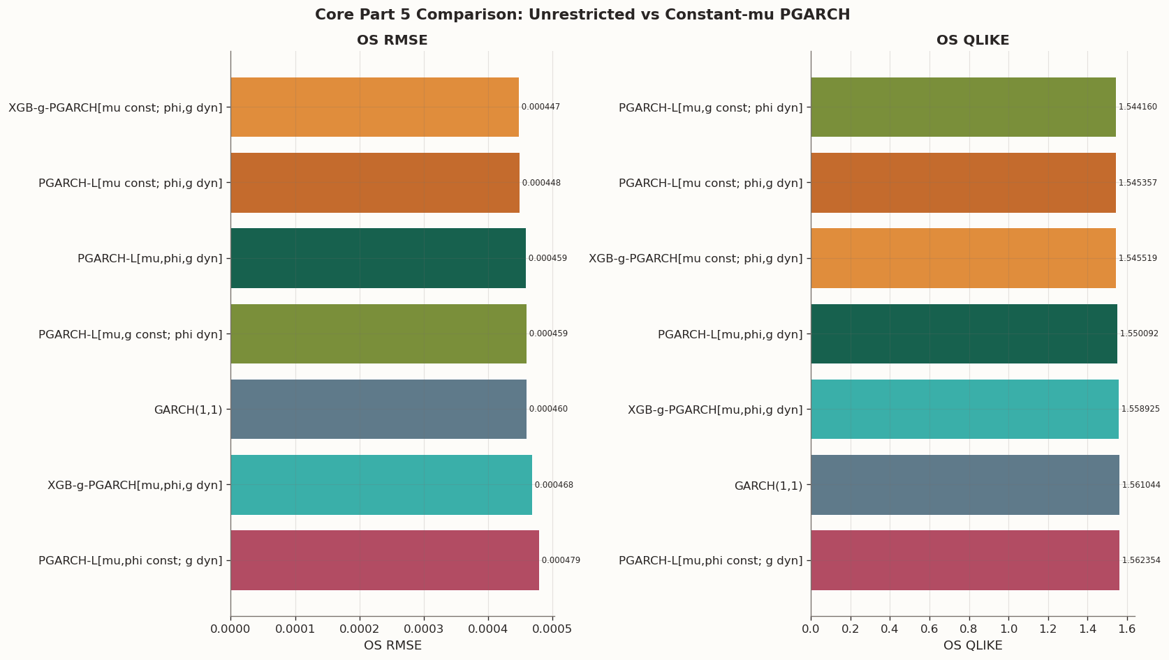
Core Part 5 comparison on the fixed three-feature protocol
OS RMSE
OS QLIKE
DM vs GARCH
p vs GARCH
Evidence
Role
Model
GARCH(1,1)
0.000460
1.561044
nan
nan
benchmark
benchmark
PGARCH-L[mu,phi,g dyn]
0.000459
1.550092
-0.422467
0.672729
directional improvement
comparison specification
XGB-g-PGARCH[mu,phi,g dyn]
0.000468
1.558925
-0.086575
0.931018
similar to benchmark
boosted comparison
PGARCH-L[mu const; phi,g dyn]
0.000448
1.545357
-1.364132
0.172677
directional improvement
main structural specification
XGB-g-PGARCH[mu const; phi,g dyn]
0.000447
1.545519
-1.352483
0.176371
directional improvement
boosted comparison
PGARCH-L[mu,phi const; g dyn]
0.000479
1.562354
0.173305
0.862429
weaker on this split
diagnostic restriction
PGARCH-L[mu,g const; phi dyn]
0.000459
1.544160
-2.624103
0.008753
directional improvement
diagnostic restriction
QLIKE and the DM test remain the primary comparison tools in Part 5. RMSE is reported as a secondary scale diagnostic. The Evidence and Role columns summarize, respectively, the forecast evidence on this split and the reason each specification appears in the comparison.
The constant-\mu family improves interpretability without requiring a forecasting sacrifice on this sample split. The constant-\mu linear model, PGARCH-L[mu const; phi,g dyn], improves mean out-of-sample QLIKE from 1.550 for the unrestricted linear model, PGARCH-L[mu,phi,g dyn], to 1.545, and it also improves RMSE from 0.000459 to 0.000448. The DM comparison against GARCH(1,1) remains directional rather than significant at conventional levels, so holding the long-run anchor fixed gives a cleaner specification while preserving benchmark-level forecast quality.
The constant-\mu boosted-g model, XGB-g-PGARCH[mu const; phi,g dyn], lands almost exactly on top of the constant-\mu linear model. This is expected and worth understanding precisely, because the same mechanism recurs in Part 6.
The gblinear booster can only add a linear correction to the g-channel raw scores, but the PGARCH-L initialiser has already found the approximately optimal linear map from the same three features to g. At that optimum the adjoint gradient with respect to g is near zero, so the booster has no signal to learn from. We verified this directly: even sweeping reg_lambda from 1.0 down to 0.001, the booster margin remains constant across all rows (zero feature-dependent variation). The residual gradient simply does not exist in the linear function class.
A separate but reinforcing mechanism is the small-Hessian problem documented in Part 3. The PGARCH recursion propagates second-order curvature through a chain of persistence factors \rho_t = \phi_t(1 - g_t), reducing per-row Hessians to O(10^{-5}) even after scaling returns by 100. The total Hessian across all training rows sums to approximately 0.09 — well below standard regularisation thresholds. We set reg_lambda= 0.01 rather than the default 1.0 to give the booster a fair chance; at \lambda = 1.0 the coordinate-descent denominator H_j + \lambda would be dominated by \lambda, masking the linear-on-linear identity behind a regularisation artefact. With \lambda = 0.01 the booster has every opportunity to learn, yet it finds nothing — confirming that the equivalence is structural, not an artefact of over-regularisation.
The equivalence would break only if the booster used a nonlinear learner (gbtree) or if a richer feature set left residual structure that the joint PGARCH-L optimisation did not fully resolve. Part 6 tests both of these directions. The unrestricted boosted-g model remains a useful comparison specification, but it is not the cleanest structural interpretation available under this information set.
The diagnostic \phi-only restriction, PGARCH-L[mu,g const; phi dyn], gives the lowest mean QLIKE in this pass and outperforms GARCH(1,1) under the DM test on this split. This restriction was added only to locate where the useful adaptation appears after fixing \mu. Time-varying persistence appears to carry more of the useful variation than a dynamic long-run anchor does in this three-feature design.
Pairwise QLIKE comparisons among the unrestricted and constant-mu PGARCH variants
OS QLIKE (A)
OS QLIKE (B)
DM (QLIKE)
p-value
Comparison
PGARCH-L[mu const; phi,g dyn] vs PGARCH-L[mu,phi,g dyn]
1.545357
1.550092
-0.221511
0.824717
XGB-g-PGARCH[mu const; phi,g dyn] vs XGB-g-PGARCH[mu,phi,g dyn]
1.545519
1.558925
-0.662636
0.507639
PGARCH-L[mu,phi const; g dyn] vs PGARCH-L[mu const; phi,g dyn]
1.562354
1.545357
1.860948
0.062896
PGARCH-L[mu,g const; phi dyn] vs PGARCH-L[mu const; phi,g dyn]
1.544160
1.545357
-0.122546
0.902478
The pairwise DM table shows that the constant-\mu linear model beats the unrestricted linear model directionally, but the improvement is small relative to sampling noise on this single split. The same is true when the unrestricted and constant-\mu boosted-g models are compared. Nevertheless, the constant-\mu extension is more interpretable than the unrestricted PGARCH-L, albeit not producing statistical gain against GARCH(1,1).
The more informative pairwise checks are the diagnostic restrictions inside the constant-\mu family. The g-only restriction, PGARCH-L[mu,phi const; g dyn], trails the constant-\mu linear model and sits close to the GARCH(1,1) benchmark, which suggests that a dynamic shock-loading channel on its own is not enough. By contrast, the \phi-only restriction, PGARCH-L[mu,g const; phi dyn], is essentially tied with the constant-\mu linear model. Taken together, those two comparisons point in the same direction: under the three return feature information set, most of the useful adaptation seems to come from time-varying persistence, while a separately dynamic g_t is secondary and a dynamic \mu_t is the least convincing channel structurally.
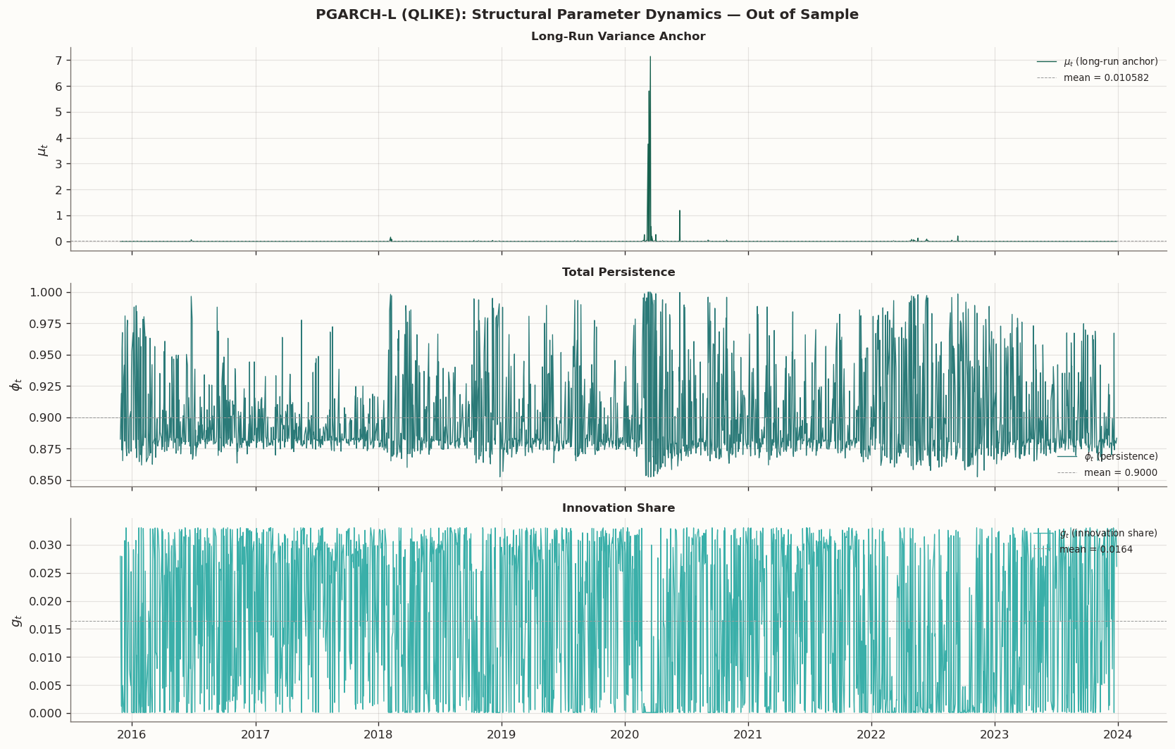
6 Diagnostics
The next table and plots compare how the unrestricted and constant-\mu linear PGARCH specifications allocate variation across the three channels on the test window. In the plot legends below, we shorten the labels to all dynamic, mu fixed, g dynamic only, and phi dynamic only. This is the direct check of whether the new family is actually more interpretable, rather than merely competitive in average loss.
Out-of-sample channel summaries for the linear PGARCH variants
mu mean
mu std
phi mean
phi std
g mean
g std
Model
PGARCH-L[mu,phi,g dyn]
0.010790
0.226838
0.899862
0.034304
0.016483
0.013223
PGARCH-L[mu const; phi,g dyn]
0.002497
0.000000
0.996399
0.038024
0.120426
0.093304
PGARCH-L[mu,phi const; g dyn]
0.013379
0.000000
0.999860
0.000000
0.123143
0.058816
PGARCH-L[mu,g const; phi dyn]
0.000141
0.000000
0.983208
0.025070
0.115163
0.000000
The unrestricted linear model assigns substantial variation to the long-run anchor: on the test window \mu_t ranges from essentially zero to several orders of magnitude above the fixed-anchor alternatives. That is hard to reconcile with the interpretation of \mu_t as a long-run variance level when the only inputs are recent return transforms.
Once \mu is fixed, the adjustment moves into \phi_t and, to a lesser extent, g_t. The near tie between the \phi-only restriction and the constant-\mu linear model, together with the weaker g-only restriction, suggests that persistence is doing most of the useful work here. We will see that more clearly in the charts below.
Compare the test-window channel paths for the unrestricted and constant-mu linear PGARCH variants
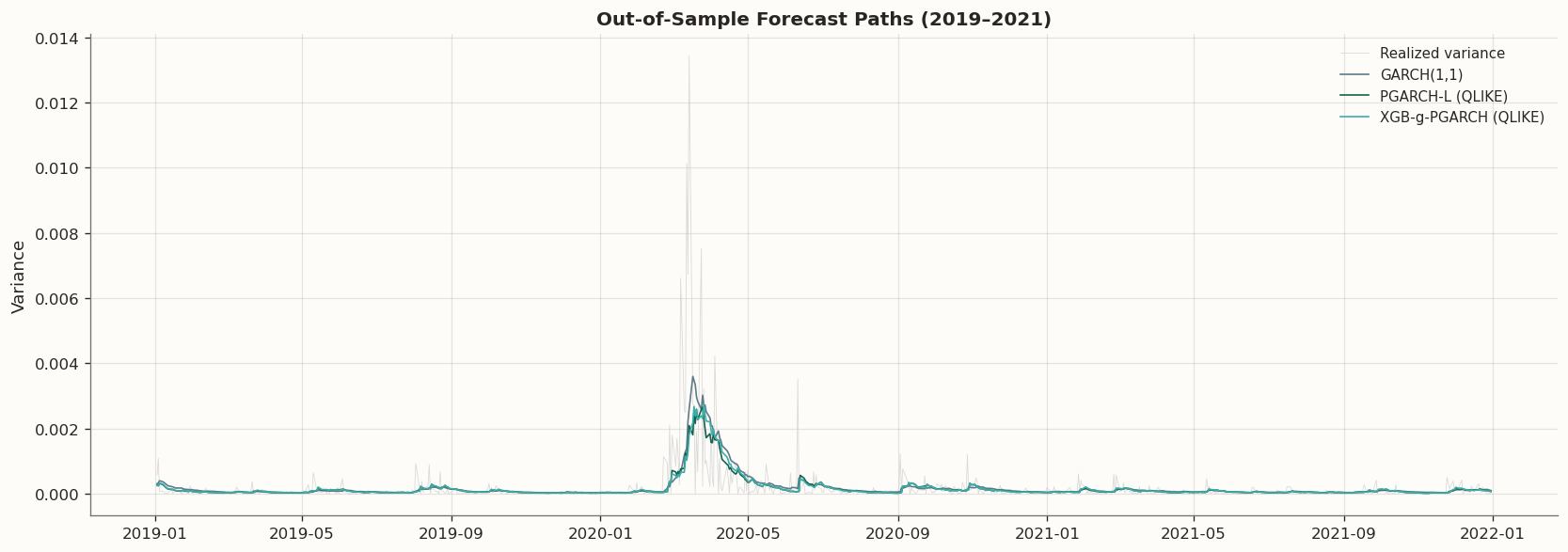
Drawing from our work in Part 4 where GARCH(1,1) has a lower QLIKE Loss than our STES-family models, we explore the structural advantage of GARCH and moves to generalize its parameters from a constant to other functional form, resulting in an unrestricted PGARCH model. However, we immediately see the problem with blindly applying our three return features to explain all the reparametrized GARCH parameters. Our return features are too fast to model the slow-moving dynamic of long-run variance level \mu. We therefore test imposing different restrictions on the PGARCH model. Within the constant-\mu family, the evidence points more toward time-varying persistence than toward time-varying shock loading alone.
The three-feature PGARCH idea remains promising. Several PGARCH variants match or beat GARCH(1,1) on mean out-of-sample QLIKE. With only lagged return, lagged absolute return, and lagged squared return available, a dynamic long-run anchor is not cleanly identified. The constant-\mu PGARCH variants therefore are the better formulation.
If the goal is a genuinely dynamic long-run channel, the information set has to change. Richer realized-volatility, calendar, or market-state features are needed before a time-varying \mu_t can be interpreted as more than a repackaging of recent shocks. Part 6 of this series is therefore motivated not by a need to discard the Part 5 PGARCH decomposition, but by the need to give its long-run channel a more credible set of predictors.
Stay tuned.
8 Appendix: PGARCH Derivative Details
This appendix collects the unrestricted PGARCH derivative formulas used in the model code. The constant-\mu and other channel-restricted variants in the main text are obtained by fixing the non-intercept feature coefficients of the corresponding channel at zero while retaining the intercept term, so no new derivative machinery is required.
8.1 Loss functions
We consider two training losses over the effective sample t = 1, \ldots, T-1 (excluding the warm-start h_0), with N = T-1:
Let \theta = [w_\mu, w_\phi, w_g] and \tilde{x}_{t-1} = [1, x_{t-1}]. Define block-embedded vectors d_t^\mu, d_t^\phi, d_t^g that place \tilde{x}_{t-1} in the appropriate block of \theta and zeros elsewhere.