Volatility Forecasts (Part 7 - Stress Testing a Benchmark-Clearing Specification)
2026-03-17
1 Introduction
Part 6 established the key obstacle on the expanded feature tier: the PGARCH-family models available at that stage did not beat GARCH(1,1) under the fixed Diebold-Mariano comparison on QLIKE loss. We decided that . That was an important result — the first time any model in this series cleared the GARCH(1,1) benchmark on the expanded-feature design — but it was not yet a publication-ready one.
This notebook is a stress-test pass rather than a fresh model search. The goal is to sharpen the claim, understand the mechanism, and decide which branch is genuinely worth expanding next. In particular, we want to know whether the gain comes from nonlinear recursion itself, from disciplined initialization, from feature compression, or from some interaction of those ingredients.
The stress test runs four branches:
Top-K sweep — does the gain depend on the exact shortlist width, or is it stable across nearby screen sizes?
Feature-selection stability — is the shortlist structurally meaningful or mainly a one-window artefact?
Rolling robustness — does the benchmark-clearing result survive when the train/test boundary shifts?
Channel ablation and screened linear diagnostic — where does the gain actually live — in the nonlinear tree layer, or in the feature compression that precedes it?
2 Evaluation Standard and Experimental Design
The acceptance standard carries over from Parts 5 and 6:
Dataset: SPY next-day squared-return, 2000–2023.
Feature tier: the same 73-column expanded feature design cached from Part 6.
where \mu_t > 0 is the long-run variance anchor, \phi_t \in (0,1) controls total persistence, and g_t \in (0,1) governs the innovation share. The implied standard GARCH parameters are \omega_t = (1 - \phi_t)\mu_t, \alpha_t = \phi_t g_t, \beta_t = \phi_t(1-g_t), with \alpha_t + \beta_t = \phi_t < 1 enforced by construction.
2.2 Stress-Test Branches
Branch
Description
Key Change
Hypothesis
Top-K sweep
Rerun the XGBPGARCH recipe at K \in \{10, 15, 20, 25, 30\}
Width of the screened feature set
Best performance concentrates in a narrow K-band, supporting a bias-variance story
Feature-selection stability
Recompute the PGARCH-based ranking on five expanding windows inside training
Window endpoint
A stable core of features survives across windows
Rolling robustness
Evaluate the recipe on five causal OOS blocks with rolling 4000-row train windows
Train/test boundary
The benchmark-clearing result is not a one-split artefact
Channel ablation + screened PGARCH
Ablate which nonlinear channels (\mu, \phi, g) are active; compare screened linear PGARCH on the same subsets
Architectural complexity
The gain lives in screening and regularisation, not in the tree layer itself
Utility functions: data loading, model fitting, loss computation
The bounded search did identify a credible benchmark-clearing XGBPGARCH specification, and the stress test confirms that the gain is real. The key revision from the stress test is interpretive: the strongest current results come from compact screened PGARCH-style models, and the present notebook does not yet show that tree-based nonlinearity is the essential driver.
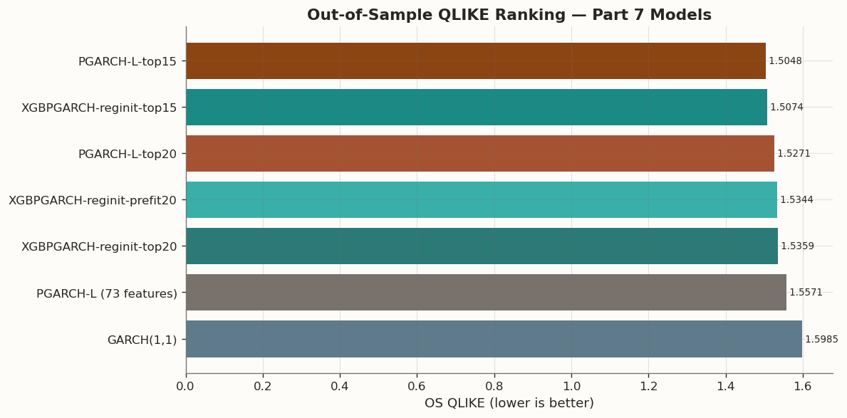
The combined result table below collects the headline models from the original bounded search, the top-K sweep, and the screened linear diagnostic.
_palette_map = {'GARCH(1,1)': '#5F7A8A','PGARCH-L (73 features)': BLOG_PALETTE[3],'XGBPGARCH-reginit-prefit20': '#3AAFA9','XGBPGARCH-reginit-top15': '#1B8A84','XGBPGARCH-reginit-top20': '#2B7A78','PGARCH-L-top15': BLOG_PALETTE[0],'PGARCH-L-top20': BLOG_PALETTE[1],}chart_df = main_summary_df.sort_values('OS QLIKE', ascending=True).reset_index(drop=True)bar_colors = [_palette_map.get(m, '#999999') for m in chart_df['Model']]fig, ax = plt.subplots(figsize=(10, 5))bars = ax.barh(chart_df['Model'], chart_df['OS QLIKE'], color=bar_colors, edgecolor='white', linewidth=0.6)ax.set_xlabel('OS QLIKE (lower is better)')ax.set_title('Out-of-Sample QLIKE Ranking — Part 7 Models', fontsize=13, fontweight='bold')ax.invert_yaxis()for bar, val inzip(bars, chart_df['OS QLIKE']): ax.text(val, bar.get_y() + bar.get_height() /2, f' {val:.4f}', va='center', fontsize=8)fig.tight_layout()plt.show()
4 Statistical Comparison
The ranking chart shows the point estimates; the Diebold-Mariano table below tests whether the differences are statistically significant. All comparisons use QLIKE loss differentials with horizon h = 1.
Three comparisons carry the most interpretive weight:
Screened models vs. GARCH(1,1): Both PGARCH-L-top15 and XGBPGARCH-top15 clear the benchmark. The DM statistics and p-values confirm that the improvement is statistically significant, not just a point-estimate artefact.
Screened models vs. full PGARCH-L (73 features): The screened variants also significantly outperform the full 73-feature linear PGARCH, confirming that feature compression is doing real work here.
XGBPGARCH vs. screened PGARCH-L (same K): At the same screen width, the boosted and linear variants are statistically indistinguishable. The nonlinear tree layer is not yet contributing a detectable margin over the regularised linear recursion.
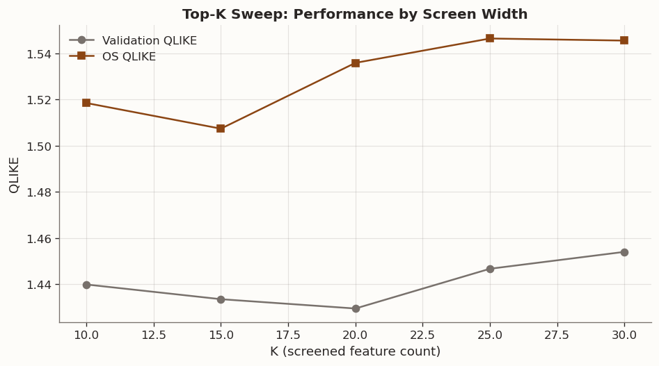
5 Top-K Sweep
The first stress test asks whether the original top-20 shortlist is special, or whether there is a stable performance band around it. The ranking protocol is recomputed on the fit split only using a regularised PGARCH coefficient norm, then the winning XGBPGARCH recipe is rerun at K \in \{10, 15, 20, 25, 30\}.
Performance peaks in a narrow band around K = 15, with the best validation and OS QLIKE concentrated there. Performance is still competitive at K = 10 and K = 20, but degrades once the screened set widens to 25 or 30 features.
That pattern strongly supports the feature-compression interpretation. If more predictors were uniformly helpful once nonlinearity was available, performance should improve or at least remain flat as K increases. Instead, the useful signal is concentrated in a compact subset.
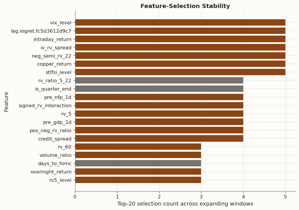
6 Feature-Selection Stability
Is the shortlist structurally meaningful or mainly a one-window accident? The same ranking rule is recomputed on five expanding windows that stay entirely inside the training segment used for selection.
Feature-selection frequency across expanding windows
plot_df = stability_freq_df.head(20).sort_values( ['selection_count', 'mean_rank'], ascending=[True, False])bar_colors = [BLOG_PALETTE[0] if flag else BLOG_PALETTE[3] for flag in plot_df['in_original_top20']]fig, ax = plt.subplots(figsize=(8.5, 6.0))ax.barh(plot_df['feature'], plot_df['selection_count'], color=bar_colors, edgecolor='white', linewidth=0.4)ax.set_xlabel('Top-20 selection count across expanding windows')ax.set_ylabel('Feature')ax.set_title('Feature-Selection Stability', fontsize=12, fontweight='bold')fig.tight_layout()plt.show()
The shortlist is not perfectly rigid, but it is far from random. Several features — including vix_level, intraday_return, iv_rv_spread, neg_semi_rv_22, copper_return, and stlfsi_level — appear in every top-20 resample. The instability is concentrated in the margin of the list rather than in the core.
That matters: the screened branch is anchored by a stable core of volatility-level, return-decomposition, and stress-sensitive predictors, even though the last few slots in the shortlist rotate. This is evidence for meaningful structure, and also a reason to be cautious about treating any single K = 20 list as canonical.
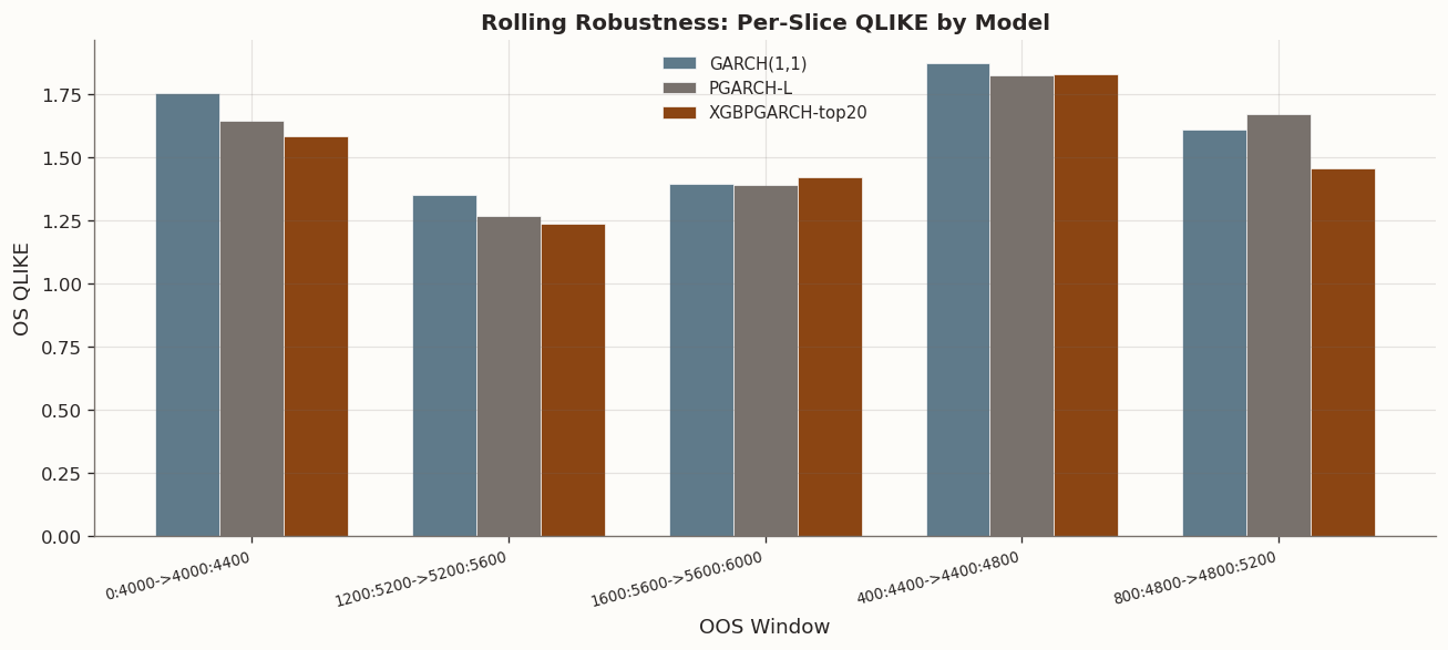
7 Rolling Robustness
A benchmark-clearing result on one fixed OOS segment is not enough on its own. The rolling robustness check holds the screened XGBPGARCH recipe fixed and evaluates it on five causal OOS blocks, each using a past-only 4000-row train window.
GARCH(1,1) does not win any of the five blocks. The screened XGBPGARCH recipe wins several blocks, while PGARCH-L contends for the others. That is enough to reject the hypothesis that the original result was a one-split artefact, but not enough to claim uniform dominance of any single architecture.
The honest reading is intermediate: screened PGARCH-style models appear to survive across multiple volatility regimes and repeatedly beat the univariate benchmark. Robustness exists at the family level more clearly than at the exact XGB architecture level.
8 Channel Decomposition
The structural ablation starts from the screened XGB specification and asks whether the gain lives in nonlinear updates to \mu, \phi, g, or in their interaction. The follow-up screened linear diagnostic then tests whether any of that nonlinearity is even needed.
The ablation outcome is unusually informative because it is flat. Every nonlinear channel configuration lands on the same score. That is not evidence that all channels matter equally — it is evidence that, under the current regularisation and tree budget, the nonlinear layer is not visibly adding differentiated value.
The screened linear diagnostic resolves the ambiguity. Once the same top-15 and top-20 subsets are passed through plain regularised PGARCH-L, the linear screened models match or outperform the boosted versions on this split. The present mechanism story is therefore feature compression plus regularised PGARCH recursion, with the nonlinear tree layer still unproven as the essential margin.
9 Diagnostic Plots
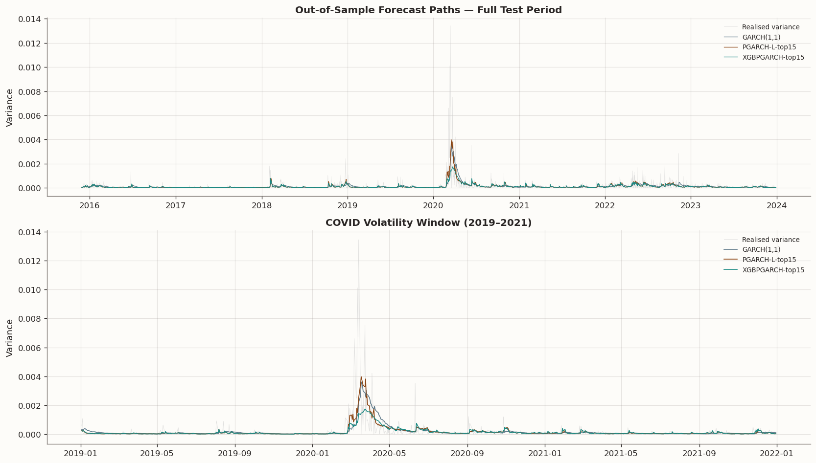
9.1 Forecast Overlay
The time-series overlay below shows realised variance against the three key forecasts on the full OOS period. The zoom highlights the COVID volatility spike, where structural differences between models are most visible.
Forecast paths: realised vs GARCH vs PGARCH-L-top15 vs XGBPGARCH-top15
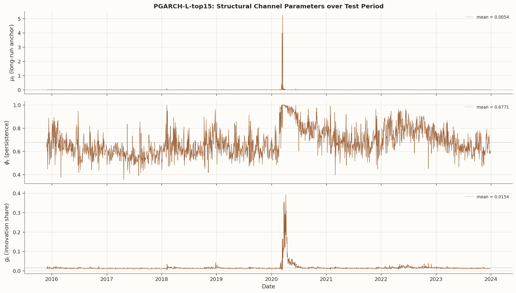
The three-panel plot below shows the time-varying structural parameters of the screened PGARCH-L-top15 over the test period. These channels correspond to the long-run variance anchor (\mu_t), total persistence (\phi_t), and innovation share (g_t).
The Mincer-Zarnowitz regression y_t = \alpha + \beta\,\hat h_t + \varepsilon_t tests whether a forecast is well calibrated. A perfectly calibrated forecast has \beta = 1 and high R^2.
The table below reports the mean and standard deviation of the implied GARCH-form parameters (\omega_t, \alpha_t, \beta_t) for the screened PGARCH-L models, alongside the static GARCH(1,1) estimates for reference.
Implied GARCH parameters for screened PGARCH-L models
Three pieces of information matter more than the headline win itself.
The initialiser failure is substantive. The built-in linear_pgarch initialiser inside XGBPGARCHModel repeatedly failed on the 73-feature design because the internal unregularised linear PGARCH fit hit the optimiser limit. The unconstrained high-dimensional starting point is brittle before any tree-based nonlinear update is even applied.
The all-feature nonlinear model collapsing back toward the full PGARCH-L reference is informative. If unrestricted nonlinear capacity were the main missing ingredient, repairing the initialiser and letting all 73 features through should have been enough. It was not. The all-feature nonlinear branch sits close to the linear PGARCH result — a clear indicator that dimensionality, not architecture, is the binding constraint.
The narrower screened branches are more interesting than an unrestricted win. Once the feature set is compressed into a compact subset, performance improves sharply. The screened linear diagnostic confirms that PGARCH-L-top15 can match or outperform the boosted specification on the same features. At this stage the cleanest mechanism story is feature compression plus regularised PGARCH recursion, with the nonlinear tree layer still unproven as the essential margin.
11 Limitations
This notebook now contains credible benchmark-clearing results, but two cautions remain.
The first is statistical: the main benchmark-clearing result still lives on a single fixed OOS segment, even though the rolling follow-up is informative. A stronger claim would require out-of-sample evaluation on data not available during any stage of the search or stress test.
The second is structural: once the screened linear PGARCH diagnostic is included, the current evidence no longer supports a clean “nonlinearity beats GARCH” narrative. It supports a narrower “screened PGARCH-style models beat GARCH on this design” story. The VolGRU branch remains pruned for this feature tier — none of the new evidence suggests that missing hidden-state dynamics are the current bottleneck.
12 Where To Go Next
Build a stability-aware screened PGARCH branch. The top-K sweep peaks in the 10–15 band, and the stability analysis shows a clear core of repeatedly selected features. The next experiment should fit PGARCH-L on a stability-aware shortlist — the intersection of the high-frequency features plus a small rotating margin.
Run a focused regularisation sweep inside screened linear PGARCH. The stress test suggests that screening and regularisation are doing more work than the tree layer. The next step should vary \lambda_\mu, \lambda_\phi, and \lambda_g around the current uniform 0.01 setting, but only inside the best K band.
Revisit nonlinearity only from the screened linear baseline. The flat ablation says the current boosted layer is not yet the decisive ingredient. If nonlinearity is revisited, it should start from the screened linear branch and change only one thing at a time: higher tree budget, milder shrinkage, or a g-only nonlinear update with the linear \mu and \phi channels frozen.
Make the rolling branch stability-aware. Test whether the stable-core shortlist travels better across windows than a single fixed selected set.
13 Conclusion
Part 7 does two jobs at once. It identifies benchmark-clearing specifications on the expanded feature tier, and it shows why the first tempting explanation — “the nonlinear model wins” — is too loose.
The bounded search result remains real: a carefully initialised and regularised XGBPGARCH branch can beat GARCH(1,1) on the fixed Part 7 split. The stress-test evidence says the cleaner and more defensible story is narrower. The strongest current results come from compact screened PGARCH-style models, and the present notebook does not yet show that tree-based nonlinearity is the essential driver.
That is still progress. A benchmark-clearing specification has been found, the active research branch is now better defined, and the next task is no longer merely to search for a winner. It is to understand why the screened branch works, how robust it is, and whether any added nonlinear capacity survives that stricter standard.