Expected Performance of a Mean-Reversion Trading Strategy - Part 3
2026-03-02
In Part 1 we derived the asymptotic Sharpe ratio \mathrm{SR}_\infty = \sqrt{\theta/2} for a mean-reversion strategy with perfect knowledge of fair value, and Part 2 showed that a constant bias M in the fair-value estimate leaves expected PnL untouched while increasing path risk, producing a penalty factor (1 + \xi^2)^{-1/2} where \xi = M/s_\infty is the bias measured in units of the stationary mispricing scale s_\infty = \sigma/\sqrt{2\theta}.
1 Random Independent Bias
Before tackling correlated estimation error, it is useful to verify that the Part 2 penalty formula extends to a random bias drawn independently of the price process. Suppose the trader’s bias M is sampled once from a distribution F with \mathbb{E}[M]=0 and \mathbb{E}[M^2] = \sigma_M^2, independently of the Brownian motion \{W_t\}. Each realisation of M is a constant over the trading period, so conditionally on M the PnL is exactly the Part 2 expression:
Y_t = \frac{\sigma^2 t - X_t^2}{2} + M X_t.
Since M and X_t are independent and \mathbb{E}[X_t] = 0, the expected PnL is unchanged:
\mathbb{E}[Y_t] = \frac{\sigma^2 t - s_t^2}{2}.
For path risk, the quadratic variation d\langle Y\rangle_t = \sigma^2(X_t - M)^2\,dt gives, by the law of iterated expectation:
This is identical to Part 2’s formula with M^2 replaced by \mathbb{E}[M^2] = \sigma_M^2. (Note that \sigma_M^2 here denotes the second moment \mathbb{E}[M^2], which equals \operatorname{Var}(M) only because \mathbb{E}[M] = 0. If the bias had a nonzero mean, the penalty would depend on the full second moment \operatorname{Var}(M) + (\mathbb{E}[M])^2.) Using the stationary mispricing scale s_\infty = \sigma/\sqrt{2\theta} from Part 2, the asymptotic Sharpe ratio follows immediately:
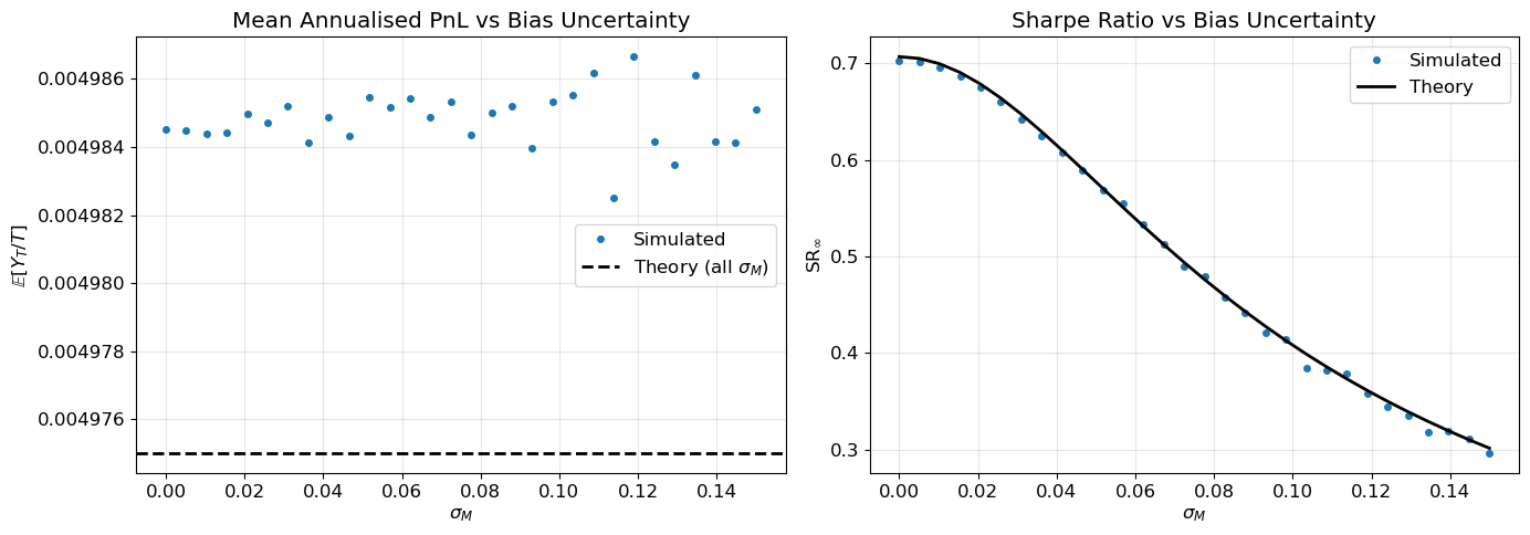
The conclusion reinforces Part 2: uncertainty in fair value increases path risk without affecting the expected return, and the Sharpe penalty depends only on \mathbb{E}[M^2], regardless of the shape of F. Figure 1 confirms both predictions via Monte Carlo. The independence assumption, however, is the crucial one. As we show next, relaxing it changes the picture qualitatively.
Show simulation code
# --- Simulation: SR with random independent bias ---theta, sigma, T, dt =1.0, 0.10, 100, 1/252n_paths =3_000X = simulate_ou(theta, sigma, T, dt, n_paths)sigma_M_values = np.linspace(0, 0.15, 30)rng_M = np.random.default_rng(99)mean_pnls, sr_sim = [], []for sm in sigma_M_values: M_draw = rng_M.normal(0, sm, size=n_paths) if sm >0else np.zeros(n_paths) Y = pnl_paths(X, M_draw, dt) mean_pnl = (Y[:, -1] / T).mean() mean_pnls.append(mean_pnl) dX = np.diff(X, axis=1) dY =-(X[:, :-1] - M_draw[:, None]) * dX qv = np.sum(dY**2, axis=1) sr_sim.append(mean_pnl / np.sqrt((qv / T).mean()))fig, axes = plt.subplots(1, 2, figsize=(14, 5))# Left: mean annualised PnL vs sigma_M (should be flat)theory_mean =0.5* (sigma**2- s2(T, theta, sigma) / T)axes[0].plot(sigma_M_values, mean_pnls, "o", ms=4, label="Simulated")axes[0].axhline(theory_mean, color="k", ls="--", lw=2, label=r"Theory (all $\sigma_M$)")axes[0].set(xlabel=r"$\sigma_M$", ylabel=r"$\mathbb{E}[Y_T/T]$", title="Mean Annualised PnL vs Bias Uncertainty")axes[0].legend()# Right: SR vs sigma_M (theory + MC)sr_theory = np.sqrt(theta /2) / np.sqrt(1+2* theta * sigma_M_values**2/ sigma**2)axes[1].plot(sigma_M_values, sr_sim, "o", ms=4, label="Simulated")axes[1].plot(sigma_M_values, sr_theory, "k-", lw=2, label="Theory")axes[1].set(xlabel=r"$\sigma_M$", ylabel=r"$\mathrm{SR}_\infty$", title="Sharpe Ratio vs Bias Uncertainty")axes[1].legend()print("Left: expected PnL is invariant to bias uncertainty. Right: SR degrades with sigma_M.")plt.tight_layout()plt.show()
Figure 1: Random independent bias. Expected PnL is invariant to bias uncertainty (left). SR degrades with \sigma_M following the same penalty formula as the constant-bias case (right).
Left: expected PnL is invariant to bias uncertainty. Right: SR degrades with sigma_M.
2 Time-Varying Correlated Bias
We now allow the bias M_t to vary over time and to be correlated with the mispricing X_t. This is the practically relevant case: any estimate derived from the price history will, by construction, covary with price movements.
2.1 Expected PnL with correlated bias
The PnL decomposition from Part 2 generalises to a time-varying bias:
Y_t = \frac{\sigma^2 t - X_t^2}{2} + \int_0^t M_u\, dX_u.
The structure is the same — an unbiased piece plus a bias-induced integral — but the second term is now a genuine Itô stochastic integral rather than the simple product MX_t of the constant-bias case.
Substituting the OU dynamics dX_u = -\theta X_u\, du + \sigma\, dW_u:
The stochastic integral \int_0^t M_u\, dW_u has zero expectation by the martingale property (the integrand M_u is adapted and satisfies \mathbb{E}[\int_0^t M_u^2\, du] < \infty, which holds for all the estimators considered below). Since \mathbb{E}[X_u] = 0, we have \mathbb{E}[M_u X_u] = \operatorname{Cov}(M_u, X_u). The expected annualised PnL is therefore:
This is the central result of the post. Compared to Parts 1–2, the expected PnL acquires a correction term proportional to the time-averaged covariance between the bias and the mispricing. Positive covariance — the bias and the mispricing moving in the same direction — reduces expected PnL: when the asset is overpriced (X>0), the bias also tends to be positive, so the trader under-estimates the overpricing and takes too small a position. Negative covariance would increase expected PnL, but this requires a contrarian estimator that anticipates mean reversion, a rare luxury in practice. Zero covariance recovers the Part 2 result, confirming that independent bias affects only risk.
2.2 A contrast: proportional bias
To sharpen intuition for the EMA analysis that follows, consider the idealised case M_t = \rho\, X_t for some \rho \in [0,1). This assumes the trader has access to the true mispricing X_t — making it a theoretical benchmark rather than a realisable estimator — but it provides a clean contrast with the EMA. The trader’s perceived mispricing is then \tilde{X}_t = (1-\rho)\,X_t, and the PnL satisfies Y_t = (1-\rho)\,(\sigma^2 t - X_t^2)/2. Both the expected PnL and the path risk scale by (1-\rho) and (1-\rho)^2 respectively, so the Sharpe ratio remains \sqrt{\theta/2}, independent of \rho. Proportional bias reduces capacity without degrading risk-adjusted return — a qualitatively different outcome from the lagged, asymmetric distortion introduced by trailing estimators.
3 EMA Trailing Estimator
With the general covariance correction in hand, we now apply it to the most natural source of correlated bias: a trailing estimator of fair value. Suppose the trader estimates \tilde{v}_t by exponentially smoothing past prices:
where \lambda > 0 is the EMA decay rate. Since p_t = v + X_t (constant fair value) and \tilde{v}_t = v + M_t, the bias M_t = \tilde{v}_t - v satisfies
dM_t = \lambda\,(X_t - M_t)\,dt, \qquad M_0 = 0.
The bias is functionally determined by the path of X — its dynamics have no independent dW_t component, only a lagged response to the mispricing. The EMA half-life is \ln 2/\lambda. Unlike the proportional bias M_t = \rho X_t discussed above, the EMA introduces a temporal lag: M_t tracks X_t with delay, and this asymmetry between the bias and the mispricing is what breaks the Sharpe-ratio invariance.
3.1 Stationary moments
The joint system (X_t, M_t) is a two-dimensional linear SDE, and its stationary second moments can be derived by applying the product rule and setting time derivatives to zero. (The joint system is exponentially ergodic — both eigenvalues of the drift matrix are strictly negative — so the time-averaged moments converge to these stationary values at an exponential rate.)
For \mathbb{E}[X_t^2], Itô’s formula gives d(X^2) = (\sigma^2 - 2\theta X^2)\,dt + 2\sigma X\,dW, so in stationarity:
It is worth noting that \Sigma_{MM} = \Sigma_{XM}: the variance of the bias equals its covariance with the mispricing. This is a consequence of the deterministic dynamics of M_t — the bias has no independent noise source, so all of its variability derives from its coupling to X_t. The stationary correlation between the bias and the mispricing is
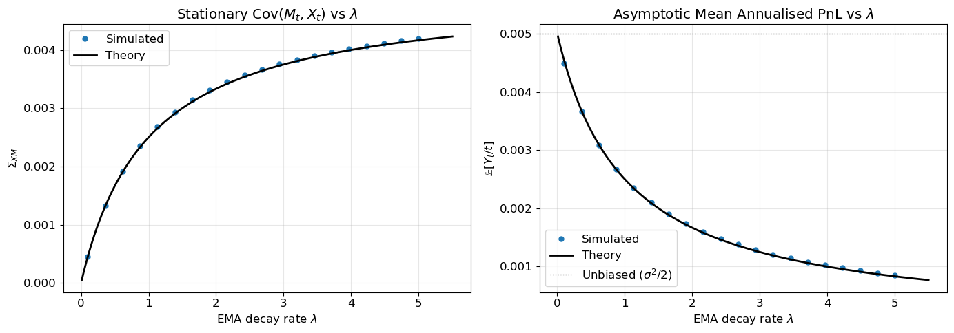
As \lambda \to \infty (fast EMA), \operatorname{Corr} \to 1 and the bias tracks the mispricing almost perfectly. As \lambda \to 0 (slow EMA), \operatorname{Corr} \to 0 and the bias decouples from the mispricing. Figure 2 confirms these stationary moments via Monte Carlo.
3.2 Asymptotic expected PnL
Substituting \Sigma_{XM} into the general covariance correction derived above:
\boxed{
\text{Asymptotic mean PnL rate}
= \frac{\sigma^2\theta}{2(\theta+\lambda)}.
}
The expected PnL is reduced by a factor \theta/(\theta+\lambda) relative to the perfect-information benchmark \sigma^2/2. At \lambda = \theta — when the EMA half-life matches the OU half-life — the expected PnL is exactly halved.
3.3 Asymptotic quadratic variation
The stationary variance of the trader’s signal \tilde{X}_t = X_t - M_t determines the path risk:
Both the numerator (expected PnL) and the denominator (path risk) of the Sharpe ratio are suppressed by the factor 1/(\theta+\lambda), but their ratio does not cancel — the square root in the denominator leaves a net penalty.
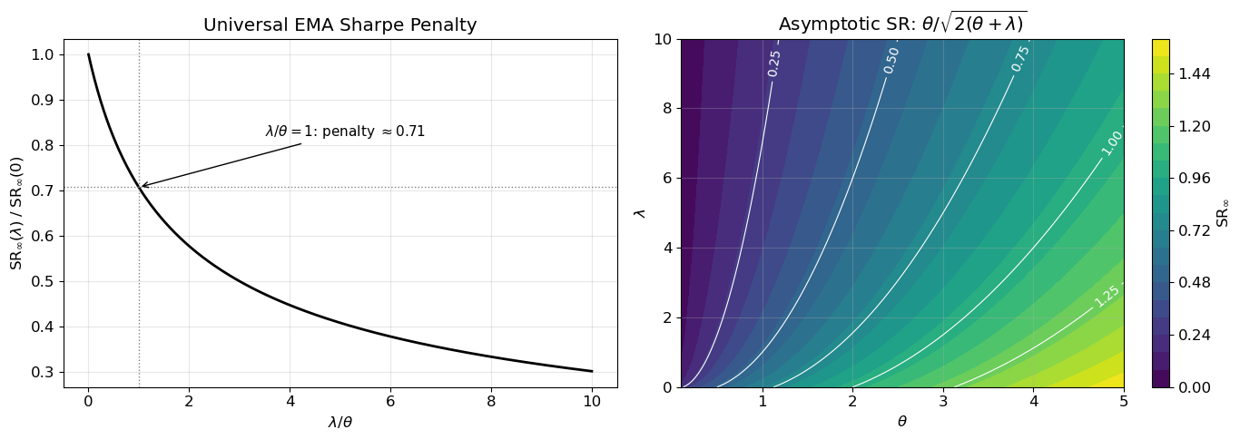
The penalty factor \sqrt{\theta/(\theta+\lambda)} depends only on the ratio \lambda/\theta. At \lambda = 0 (no estimation) we recover the Part 1 result; at \lambda = \theta the penalty is 1/\sqrt{2} \approx 0.71; and as \lambda \to \infty the EMA tracks the price too closely and the Sharpe ratio vanishes. Figure 3 and Figure 4 confirm these predictions via Monte Carlo and display the universal penalty curve.
3.5 Finite-horizon behaviour
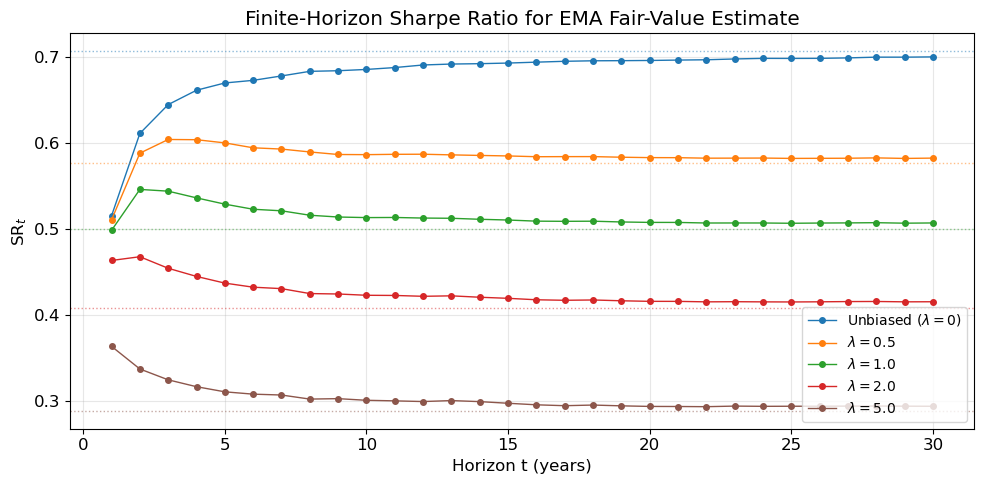
The asymptotic results above use the stationary moments of the joint system. At finite horizons, the second moments of (X_t, M_t) satisfy a 3\times 3 linear ODE (the Lyapunov equation for the system’s covariance matrix), which has closed-form exponential solutions. The resulting finite-horizon Sharpe ratio \mathrm{SR}_t involves these time-dependent moments in place of \Sigma_{XX}, \Sigma_{XM}, and \Sigma_{MM}. Figure 5 shows the convergence of \mathrm{SR}_t to the asymptotic limit for several EMA decay rates; the exponential ergodicity of the joint system ensures convergence is rapid once t exceeds a few multiples of the longer time-scale 1/\min(\theta, \lambda).
Figure 2: Stationary covariance and expected PnL vs EMA decay rate. Theory (solid lines) uses the closed‐form expressions; dots are Monte Carlo estimates.
Unbiased PnL rate: 0.0050. At lambda=theta=1.0: 0.0025 (halved).
Show simulation code
# --- SR vs theta for different EMA speeds ---sigma =0.10T, dt, n_paths =100, 1/252, 1_000theta_range = np.linspace(0.1, 5.0, 30)lam_values = [0.0, 0.5, 1.0, 2.0]fig, ax = plt.subplots(figsize=(10, 6))colors = plt.cm.tab10(np.linspace(0, 0.4, len(lam_values)))for lam, c inzip(lam_values, colors):# Theory curveif lam ==0: sr_th = np.sqrt(theta_range /2) label =r"Unbiased ($\lambda=0$)"else: sr_th = theta_range / np.sqrt(2* (theta_range + lam)) label =f"$\\lambda={lam}$" ax.plot(theta_range, sr_th, "-", color=c, lw=2, label=f"Theory {label}")# MC at subset of theta values theta_sim = theta_range[::5] sr_sim = []for th in theta_sim: seed_rng = np.random.default_rng(123)if lam ==0: X = simulate_ou(th, sigma, T, dt, n_paths, rng=seed_rng) M_arr = np.zeros_like(X)else: X, M_arr = simulate_ou_ema(th, sigma, lam, T, dt, n_paths, rng=seed_rng) Y = pnl_paths(X, M_arr, dt) mean_pnl = (Y[:, -1] / T).mean() dX = np.diff(X, axis=1) dY =-(X[:, :-1] - M_arr[:, :-1]) * dX qv = np.sum(dY**2, axis=1) sr_sim.append(mean_pnl / np.sqrt((qv / T).mean())) ax.plot(theta_sim, sr_sim, "o", color=c, ms=7, zorder=5)ax.set(xlabel=r"Mean reversion speed $\theta$", ylabel="Asymptotic Sharpe Ratio", title=r"Sharpe Ratio vs $\theta$ for EMA Fair-Value Estimate (dots = MC)")ax.legend(loc="upper left")plt.tight_layout()plt.show()
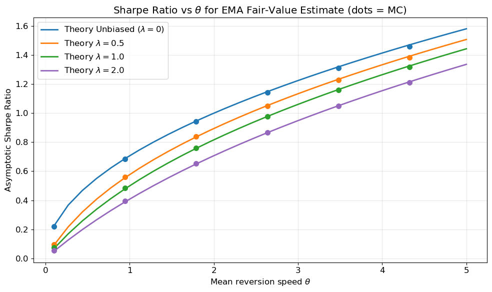
Figure 3: Sharpe ratio vs \theta for different EMA decay rates. Lines are the closed-form \theta/\sqrt{2(\theta+\lambda)}; dots are Monte Carlo estimates.
Figure 4: Left: the Sharpe-ratio penalty () depends only on the ratio (/). Right: the absolute asymptotic Sharpe ratio (/) over the ((,)) plane.
Left: penalty depends only on lambda/theta. Right: absolute SR over the (theta, lambda) plane.
4 All Linear Trailing Estimates Create Positive Correlation
The EMA penalty derived above is not specific to exponential weighting — it is an instance of a general result for linear estimators with non-negative kernels. Any trailing estimator of the form
For the OU process, the autocovariance \operatorname{Cov}(X_s, X_t) = s_s^2\, e^{-\theta(t-s)} is everywhere non-negative for s \leq t. Since both w and the autocovariance are non-negative, the integral is non-negative — and strictly positive unless w = 0 almost everywhere, which corresponds to no estimation at all.
The EMA corresponds to exponential weights w(u) = \lambda e^{-\lambda u}; a simple moving average over a window \tau uses rectangular weights w(u) = 1/\tau for u \in [0,\tau]. In every case, the trailing estimate injects positive correlation, and the expected PnL falls below the perfect-information benchmark \sigma^2/2. The positive-correlation penalty is therefore not a modelling artefact of the EMA but an unavoidable cost of inferring fair value from price history via any linear estimator with non-negative weights. (Non-linear or sign-changing estimators could in principle achieve negative bias–mispricing covariance, but at the cost of introducing other distortions.) Figure 5 illustrates the finite-horizon convergence of the Sharpe ratio for several EMA decay rates.
Figure 5: Finite-horizon Sharpe ratio convergence for EMA fair-value estimates with different decay rates. Dotted horizontal lines show the asymptotic limits.
5 Discussion
The key distinction established in this post is between independent and correlated estimation error. An independent bias — whether constant or random — leaves the expected PnL untouched and degrades only risk, exactly as in Part 2 (Figure 1). A correlated bias, by contrast, directly reduces the expected return through the covariance correction -(\theta/t)\int_0^t \operatorname{Cov}(M_u, X_u)\,du, as demonstrated for the EMA trailing estimator in Figure 2. The mechanism is intuitive: when the trader’s fair-value estimate co-moves with the price, the estimate chases the price rather than anchoring to true value, weakening the mean-reversion signal at its source.
The EMA Sharpe penalty \sqrt{\theta/(\theta+\lambda)} = 1/\sqrt{1+\lambda/\theta} collapses to a universal curve in \lambda/\theta (Figure 4), yielding a practical rule of thumb: the EMA lookback (half-life \ln 2/\lambda) must be much longer than the OU half-life (\ln 2/\theta) — equivalently, \lambda \ll \theta — for the estimation-induced penalty to remain small. At \lambda = \theta the Sharpe ratio is roughly 71% of the unbiased level; Table 1 summarises the penalty across several values.
Table 1: EMA Sharpe penalty for selected values of \lambda/\theta.
\lambda/\theta
0
0.25
0.5
1
2
5
Penalty
1.00
0.89
0.82
0.71
0.58
0.41
The proportional-bias benchmark (M_t = \rho X_t) provides a useful contrast. In that case, both the PnL and QV scale by (1-\rho) and (1-\rho)^2 respectively, and the Sharpe ratio cancels to \sqrt{\theta/2} regardless of \rho. The EMA, however, introduces a lagged, asymmetric distortion — not a pure rescaling — and it is precisely this temporal asymmetry that degrades risk-adjusted return. The general trailing-estimate theorem then confirms that this penalty is not particular to exponential weighting: any non-negative kernel applied to an OU process produces positive correlation and therefore reduces expected PnL below the perfect-information benchmark.
6 Further directions
Several extensions of this framework merit investigation. The analysis throughout assumes a constant fair value; when v_t itself follows a random walk or trend, the OU dynamics of X_t remain valid but the assumption dp_t = dX_t breaks down, and the interplay between estimation bias and fair-value drift becomes considerably richer. A related question is the optimal choice of \lambda in the presence of trading costs: the unbiased (\lambda=0) strategy generates the highest expected PnL but relies on continuous rebalancing, and some smoothing of fair value may actually improve net performance by reducing turnover.
It is also worth noting that the EMA is not the optimal estimator of the OU mean, even within the class of linear estimators. When \theta and \sigma are known, a Kalman filter (or equivalently, the MLE for the stationary OU mean) exploits the known dynamics to produce a lower-variance estimate and a correspondingly tighter lower bound on the estimation penalty. The EMA analysis above therefore represents an achievable but not best-case scenario for trailing estimation.
On the analytical side, the EMA has the cleanest closed-form results thanks to the Markov property of the joint system, but simple moving averages and other kernel estimators are common in practice; their qualitative behaviour follows from the general trailing-estimate result above, with quantitative differences depending on the kernel shape.
In the next post we turn to a complementary source of error: uncertainty in the OU parameters \theta and \sigma themselves. Joint estimation of these parameters and fair value introduces additional correlations with the mispricing, and the rolling-estimation framework developed here will provide the analytical bridge between Parts 3 and 4.